Quantcast
Channel: Search Results for “heatmap”– R-bloggers
Viewing all 152 articles
Browse latest View live

“Digit Recognizer” Challenge on Kaggle using SVM Classification

$
0
0

(This article was first published on joy of data » R, and kindly contributed to R-bloggers)

MNIST-digitsThis article is about the “Digit Recognizer” challenge on Kaggle. You are provided with two data sets. One for training: consisting of 42’000 labeled pixel vectors and one for the final benchmark: consisting of 28’000 vectors while labels are not known. The vectors are of length 784 (28×28 matrix) with values from 0 to 255 (to be interpreted as gray values) and are supposed to be classified as to what number (from 0 to 9) it represents. The classification is realized using SVMs which I implement with kernlab package in R.

Three representation of the data set

The pre- and post-processing in all cases consists of removing the unused (white – pixel value = 0) frame (rows and columns) of every matrix and finally to scale the computed feature vectors (feature-wise) to mean 0 and standard deviation 1. I gave three representations a try:

  1. [m] Eight measurements are extracted: (ratio width/height, mean pixel value, vertical symmetry, horizontal symmetry, relative pixel weight for all four quarters).
  2. [a] Resizing to 10×10 and then just iterate through pixels by row to get a vector of length 100.
  3. [n] Dichromatize matrix. Now every black pixel can have 2^8 different neighbourhood value combinations. Each is represented in a vector of length 256 which keeps the frequency of the occurences.

To my surprise those three representations performed reverse to what I expected. Best performance showed [a], then [m] and way off was [n]. In hindsight (after “snooping” the data) it makes some sense. I expected more from [n] because I thought this representation might keep track well of details like curvature, straight lines and edges. I still think this approach is promising but probably the neighbourhood has to be increased to distance 2 and post-processed appropriately.

About the classifiers

First of all, as you know, an SVM can only classify into two categories. The classical approach for differentiation of N (10 for this application) categories is to train Nx(N-1)/2 classifiers. One classifier per unordered pair of different categories (one SVM for “0″ vs. “1″ and for “0″ vs. “2″ etc.). Later the input is then fed to all Nx(N-1)/2 classifiers and the category which got chosen most often is then considered to be the correct one. In case several categories share the maximum score one of it is chosen at random.

As for the kernels I sticked to the standards – Gaussian kernel and polynomial kernel (also linear kernel – polynomial kernal of degree = 1). The first grid search I performed for (Gaussian kernel) C x σ in {1,10,100,1000,10’000} x {1,0.1,0.01,0.001,0.0001} and for (polynomial kernel) C x deg in {1,10,100,1000,10’000} x {1,2,3,4,5}. All results are available  as CSVs on GitHub.

The grid search was performed for each parameter combination on 10 randomly sampled subsets of size 1000 using 5-fold cross validation on each and then taking the average. By doing so I tried to speed up the processing while keeping high accuracy. In hindsight I should have especially reduced the subsamples from 10 to 2 or 1, given how fast it became clear which kernel / feature combinations would do a reasonable job. And those doing a bad job took way way way longer to finish. Also the number of support vectors exploded as you would expect because the algorithm took a do-or-die attitude to fit the data.

> cor.test(result.rbfdot.a[,"t.elapsed"],result.rbfdot.a[,"cross"])

	Pearsons product-moment correlation

data:  result.rbfdot.a[, "t.elapsed"] and result.rbfdot.a[, "cross"]
t = 43.2512, df = 1123, p-value < 2.2e-16
alternative hypothesis: true correlation is not equal to 0
95 percent confidence interval:
 0.7675038 0.8114469
sample estimates:
      cor 
0.7904905 

> cor.test(result.rbfdot.a[,"t.elapsed"],result.rbfdot.a[,"SVs"])

	Pearsons product-moment correlation

data:  result.rbfdot.a[, "t.elapsed"] and result.rbfdot.a[, "SVs"]
t = 146.2372, df = 1123, p-value < 2.2e-16
alternative hypothesis: true correlation is not equal to 0
95 percent confidence interval:
 0.9716423 0.9774934
sample estimates:
      cor 
0.9747345

Especially calculations of linear kernel (polynomial of degree 1) for data representation of type [m] took forever. Which makes sense because this representation boils down to a vector of length eight which is quite dense and hence linear separability is not to be expected and the surface starts occilating to reach an optimum. But also for higher degrees polynomial kernels for this representation didn’t perform very impressing in comparison, so I just skipped it. Similar story for data representation [n] which took long to compute, while the performances where partially quite okay but still unimpressing in comparison to polynomial for [a] and Gaussian for [a] and [m] – hence I skipped the computation of [n] alltogether after few classifiers had been trained.

The final round: comparing rbfdot for [a] and [m] with polydot for [a]

The following table/matrix showes us the number of classifiers for a given data set / kernel combination which yielded a cross validation error lower than 1% and took on average less than 5 seconds to compute:

# performance.overview() is located on GitHub in scripts/helpers.r

> performance.overview(list(
  "polydot [a]" = result.polydot.a, 
  "rbfdot [a]" = result.rbfdot.a, 
  "rbfdot [m]" = result.rbfdot.m), 
   v="cross", th=0.01, v2="t.elapsed", th2=5)

            0:1 0:2 1:2 0:3 1:3 2:3 0:4 1:4 2:4 3:4 0:5 1:5 2:5
polydot [a]  25  21   7  25  15  13  25  19  20  25  16  15  20
rbfdot [a]   15  14   5  15   8   5  15  11  13  15   9   8   6
rbfdot [m]    7   0   0   0   0   0   0   0   0   0   0   0   0

            3:5 4:5 0:6 1:6 2:6 3:6 4:6 5:6 0:7 1:7 2:7 3:7 4:7
polydot [a]   0  23  20  23  20  25  20  10  25  15  15  20  20
rbfdot [a]    0  15  12  14   9  15  14   5  15  11  11   9   7
rbfdot [m]    0   0   0   8   0   0   0   0   0   0   0   0   0

            5:7 6:7 0:8 1:8 2:8 3:8 4:8 5:8 6:8 7:8 0:9 1:9 2:9
polydot [a]  25  25  15   1   3   0  15   0  14  10  25  15  17
rbfdot [a]   15  15  13   4   5   0   9   2  13  13  15  12  14
rbfdot [m]    0  25   0   0   0   0   0   0   0   0   0   7   0

            3:9 4:9 5:9 6:9 7:9 8:9
polydot [a]   8   0  13  25   0   1
rbfdot [a]    4   0  10  15   0   5
rbfdot [m]    0   0   0  25   0   0

Not just shows polydot for [a] on a whole a more promising performance. It almost seems as if the performance of rbfdot is basically a subset. In only one case rbfdot shows for [a] and categories “5″ vs. “8″  a classifier doing a better job than those found for polydot and [a] in the same case. Hence my decision to stick with polydot and data set representation of type [a] in the end.

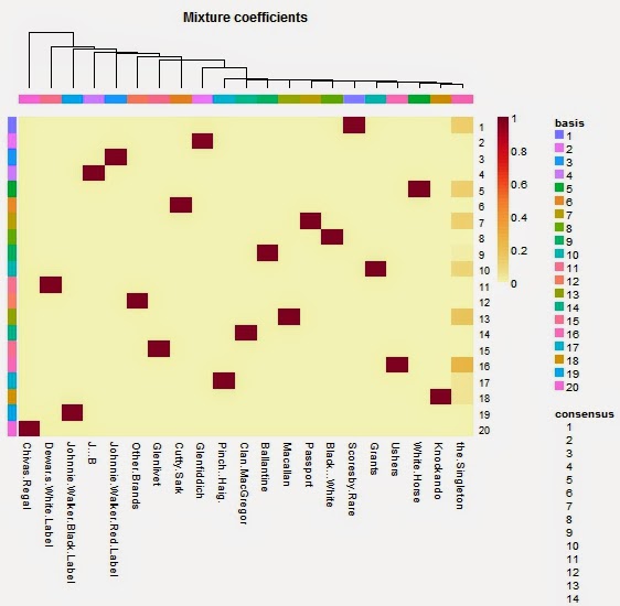
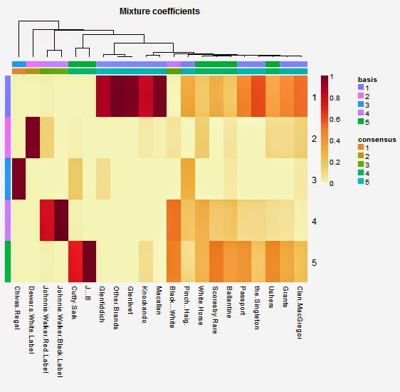
 The grids searched and found

Polynomial (normalized) Polynomial (not normalized) Gaussian (normalized)

What I am inclined to learn from those heatmaps is that on one hand optimal parameter combinations are not entirely randomly scattered all over the place but on the other hand it seems that if best performance is seeked, then one has to investigate optimal parameters individually. In this case I took the best performing classifier configurations (C and degree) with a low empirical computation time and refined C further.

And at the end of the day …

Now with the second grid search result for data set type “a” and polynomial kernel I gave it a try on the test data set and got a score of 98% plus change which landed me rank 72 of 410. The air is getting quite thin above 98% and I would have to resort to more refined data representations to improve the result. But for now I am happy with the outcome. But I guess I will sooner or later give it a second try with fresh ideas.

Expectable out of sample accuracy

expected-accuracy

I was wondering what accuracy I could expect (y-axis of the chart) from a set of classifiers (10×9/2 as ever) if I assume a homogenous accuracy (x-axis of the chart) for a classifier which is in charge of an input and a random accuracy for the others. I took several runs varying the outcome probability for the “not-in-charge-classifiers” using a normal distribution with mean 0.5 truncated to the interval 0.1 to 0.9 with different deviations. For symmetric reasons I assume that input is always of class “0″. Then f.x. all classifiers dealing with “0″ (“0″ vs. “1″, “0″ vs. “2″ etc.) will have an accuracy of say 94% and the other classifiers (“5″ vs. “7″, “2″ vs. “3″ etc.) will have an outcome probabilty between 10% and 90% with a mean of 50%. The results are surprisingly stable and indicate that for an expected accuracy of 95% an “in-charge-classifier”-accuracy of 94% is sufficient. Given that the average cross validation error of my final classifier set is more than 99% I could get in theory close to 100% for the overall accuracy. But the classifier configurations are – cross validation back and forth – still specialized to the training set and hence a lower true out of sample accuracy has to be expected. Also the assumption that the probabilities of correctness for the classifiers is not independent – simply because a “3″ is more similar to an “8″ than a “1″.

# simulate.accuracy.of.classifier.set() is located on GitHub 
# in scripts/viz-helpers.r

result.sd015 <- simulate.accuracy.of.classifier.set(10000,0.15,6)
result.sd01 <- simulate.accuracy.of.classifier.set(10000,0.1,6)
result.sd005 <- simulate.accuracy.of.classifier.set(10000,0.05,6)
result.sd001 <- simulate.accuracy.of.classifier.set(10000,0.01,6)

plot(result.sd015, xlab="avg expected accuracy of classifier if input belongs to one of its classes", 
  ylab="overall expected accuracy", pch=16,cex=.1, ylim=c(0,1))

abline(v=.94,col=rgb(0,0,0,alpha=.3))
abline(h=.95,col=rgb(0,0,0,alpha=.3))

points(result.sd01, pch=16, cex=.1, col="green")
points(result.sd005, pch=16, cex=.1, col="blue")
points(result.sd001, pch=16, cex=.1, col="orange")

for(i in 1:3) {
  result.sd015.const <- simulate.accuracy.of.classifier.set(10000,0.15,6,TRUE)
  points(result.sd015.const, pch=16, cex=.1, col="red")
}

Code and data

All scripts and the grid search results are available on GitHub. Sorry about incomplete annotation of the code. If something is unclear or you think you might have found a bug, then you are welcome to contact me. Questions, corrections and suggestions in general are very welcome.

The post “Digit Recognizer” Challenge on Kaggle using SVM Classification appeared first on joy of data.

To leave a comment for the author, please follow the link and comment on his blog: joy of data » R.

R-bloggers.com offers daily e-mail updates about R news and tutorials on topics such as: visualization (ggplot2, Boxplots, maps, animation), programming (RStudio, Sweave, LaTeX, SQL, Eclipse, git, hadoop, Web Scraping) statistics (regression, PCA, time series, trading) and more...

Heatmap of Toronto Traffic Signals using RGoogleMaps

$
0
0

(This article was first published on everyday analytics, and kindly contributed to R-bloggers)
A little while back there was an article in blogTO about how a reddit user had used data from Toronto's Open Data initiative to produce a rather cool-looking map of all the locations of all the traffic signals here in the city.

It's neat because as the author on blogTO notes, it is recognizable as Toronto without any other geographic data being plotted - the structure of the city comes out in the data alone.

Still, I thought it'd be interesting to see as a geographic heat map, and also a good excuse to fool around with mapping using Rgooglemaps.

The finished product below:


Despite my best efforts with transparency (using my helper function), it's difficult for anything but the city core to really come out in the intensity map.

The image without the Google maps tile, and the coordinates rotated, shows the density a little better in the green-yellow areas:


And it's also straightforward to produce a duplication of the original black and white figure:


The R code is below. Interpolation is using the trusty kde2d function from the MASS library and a rotation is applied for the latter two figures, so that the grid of Toronto's streets faces 'up' as in the original map.

# Toronto Traffic Signals Heat Map
# Myles Harrison
# http://www.everydayanalytics.ca
# Data from Toronto Open Data Portal:
# http://www.toronto.ca/open

library(MASS)
library(RgoogleMaps)
library(RColorBrewer)
source('colorRampPaletteAlpha.R')

# Read in the data
data <- read.csv(file="traffic_signals.csv", skip=1, header=T, stringsAsFactors=F)
# Keep the lon and lat data
rawdata <- data.frame(as.numeric(data$Longitude), as.numeric(data$Latitude))
names(rawdata) <- c("lon", "lat")
data <- as.matrix(rawdata)

# Rotate the lat-lon coordinates using a rotation matrix
# Trial and error lead to pi/15.0 = 12 degrees
theta = pi/15.0
m = matrix(c(cos(theta), sin(theta), -sin(theta), cos(theta)), nrow=2)
data <- as.matrix(data) %*% m

# Reproduce William's original map
par(bg='black')
plot(data, cex=0.1, col="white", pch=16)

# Create heatmap with kde2d and overplot
k <- kde2d(data[,1], data[,2], n=500)
# Intensity from green to red
cols <- rev(colorRampPalette(brewer.pal(8, 'RdYlGn'))(100))
par(bg='white')
image(k, col=cols, xaxt='n', yaxt='n')
points(data, cex=0.1, pch=16)

# Mapping via RgoogleMaps
# Find map center and get map
center <- rev(sapply(rawdata, mean))
map <- GetMap(center=center, zoom=11)
# Translate original data
coords <- LatLon2XY.centered(map, rawdata$lat, rawdata$lon, 11)
coords <- data.frame(coords)

# Rerun heatmap
k2 <- kde2d(coords$newX, coords$newY, n=500)

# Create exponential transparency vector and add
alpha <- seq.int(0.5, 0.95, length.out=100)
alpha <- exp(alpha^6-1)
cols2 <- addalpha(cols, alpha)

# Plot
PlotOnStaticMap(map)
image(k2, col=cols2, add=T)
points(coords$newX, coords$newY, pch=16, cex=0.3)
This a neat little start and you can see how this type of thing could easily be extended to create a generalized mapping tool, stood up as a web service for example (they're out there). Case in point: Google Fusion Tables. I'm unsure as to what algorithm they use but I find it less satisfying, looks like some kind of simple point blending:


As always, all the code is on github.

To leave a comment for the author, please follow the link and comment on his blog: everyday analytics.

R-bloggers.com offers daily e-mail updates about R news and tutorials on topics such as: visualization (ggplot2, Boxplots, maps, animation), programming (RStudio, Sweave, LaTeX, SQL, Eclipse, git, hadoop, Web Scraping) statistics (regression, PCA, time series, trading) and more...

The Current Golden Era of the NBA

$
0
0

(This article was first published on More or Less Numbers, and kindly contributed to R-bloggers)
We are in the midst of what many are calling a "golden age" of the NBA.  Being in the midst of a time where attention to the sport has seemingly increased is difficult to quantify.  For most people who have had an interest in the NBA over a long period of time, the current state of the game just "feels" like a time unlike recent years.  Awareness of the calibre of game we are witnessing is important to more fully appreciating the games and the players we get to see perform.

In the last couple of years we have seen two giants in the game emerge as contenders (Durant/Lebron) that reminds many of the Bird/Magic years.  Friendship coupled with competition in the kind of way that keeps you glued to the screen when they play.  The most valuable player (MVP) distinction, I would argue is a reasonable way to see where the game is at in terms of the quality of play in the league.  The site basketball-reference provides an enormous amount of data on the sport and is a great place to begin looking at MVP as a metric for determining the "era" of current play in the NBA.

Below is a heatmap showing different statistics gotten from the website for players that were awarded the MVP in different years.  The colors show a distribution of how the players ranked compared to eachother based on these yearly stats (Red>Blue).  On the left side of the heat map is a dendrogram showing how players could be grouped based on these stats.


The stats are total games (Games), field goal % per game (FGoalPercen), free throw % (FTPercen), assists per game (Assists), rebounds per game (Rebounds), minutes per game (Minutes), average points per game (Pts), and player age (Age).  Next we take this same dendrogram and divide players into clusters using a method (kmeans) based on the above statistics.  The red lines outline the different clusters we get when creating 5 of them.  Again these groups are based on the similarity in these stats between players.


What results is a set of data where we can see how MVPs could be grouped based on the stats in the heatmap above.  Kevin Durant hasn't been awarded the MVP yet, but let's just assume he does, and his current stats don't change at all after these 81 regular season games (this is all on a per game basis).


Clearly, cluster/group 2 or what I will call the "Golden Era Group" is the largest.  Even though some players arguable shouldn't be in this group, it's mostly comprised of players that reflective NBA watchers can agree were apart of what many have called "golden age(s)" in the NBA.  Also interesting to note are the Bill Russell and Wilt Chamberlain clusters.  In the case of Wilt Chamberlain his rebound and shooting numbers were much higher than his peers, whereas Bill Russell is placed into his own group because of his free-throw % being in the 50%-60% range...or much lower than his MVP peers.

Here are other players in the "Golden Era Group" with their Points per game against the year.  Notice how comparable Durant is to other giants in the "Golden Era", and how amazing Jordan was compared to his MVP peers.


In general, we can see that recent years' MVP awards are grouped with Bird, Magic, and Jordan.  As a proxy for measuring each players' performance in the league, measuring the performance of MVPs seems to indicate that the current level of play of the best in the NBA could be associated with these by-gone eras of greatness.  In many ways knowing that the current level of play is comparable is intuitive without looking at the numbers, just by watching the game.  In support of feeling like it's a "golden age" of the NBA there are numbers to support it.

Time for the playoffs.....


To leave a comment for the author, please follow the link and comment on his blog: More or Less Numbers.

R-bloggers.com offers daily e-mail updates about R news and tutorials on topics such as: visualization (ggplot2, Boxplots, maps, animation), programming (RStudio, Sweave, LaTeX, SQL, Eclipse, git, hadoop, Web Scraping) statistics (regression, PCA, time series, trading) and more...

Project Tycho, Correlation between states

$
0
0

(This article was first published on Wiekvoet, and kindly contributed to R-bloggers)
In this fourth post on Measles data I want to have a look at correlation between states. As described before, the data is from Project Tycho, which contains data from all weekly notifiable disease reports for the United States dating back to 1888. These data are freely available to anybody interested.

Data

I discovered an error in previous code which made 1960 to appear twice. Hence updated script.
setwd('/home/kees/Documents/tycho/')
r1 <- read.csv('MEASLES_Cases_1909-1982_20140323140631.csv',
    na.strings='-',
    skip=2)
r2 <- reshape(r1,
    varying=names(r1)[-c(1,2)],
    v.names='Cases',
    idvar=c('YEAR' , 'WEEK'),
    times=names(r1)[-c(1,2)],
    timevar='STATE',
    direction='long')
r2$STATE=factor(r2$STATE)

####################3
years <- dir(pattern='+.txt')
years

pop1 <-
    lapply(years,function(x) {
            rl <- readLines(x)
            print(x)
            sp <- grep('^U.S.',rl)
            st1 <- grep('^AL',rl)
            st2 <- grep('^WY',rl)
            rl1 <- rl[c language="(sp[1"][/c]-2,st1[1]:st2[1])]
            rl2 <- rl[c language="(sp[2"][/c]-2,st1[2]:st2[2])]
           
            read1 <- function(rlx) {
                rlx[1] <- paste('abb',rlx[1])
                rlx <- gsub(',','',rlx,fixed=TRUE)
                rt <- read.table(textConnection(rlx),header=TRUE)
                rt[,grep('census',names(rt),invert=TRUE)]
            }
            rr <- merge(read1(rl1),read1(rl2))
            ll <- reshape(rr,
                list(names(rr)[-1]),
                v.names='pop',
                timevar='YEAR',
                idvar='abb',
                times=as.integer(gsub('X','',names(rr)[-1])),
                direction='long')
        })
pop <- do.call(rbind,pop1)
pop <- pop[grep('19601',rownames(pop),invert=TRUE),]

states <- rbind(
    data.frame(
        abb=datasets::state.abb,
        State=datasets::state.name),
    data.frame(abb='DC',
        State='District of Columbia'))
states$STATE=gsub(' ','.',toupper(states$State))

r3 <- merge(r2,states)
r4 <- merge(r3,pop)
r4$incidence <- r4$Cases/r4$pop

r5 <- subset(r4,r4$YEAR>1927,-STATE)
r6 <- r5[complete.cases(r5),]

New variable

In previous posts it became clear there is in general a yearly cycle. However, the minimum in this cycle is in summer. This means for yearly summary it might be best not to use calender years, but rather something which breaks during summer. My choice is week 37.
with(r6[r6$WEEK>30 & r6$WEEK<45,],
    aggregate(incidence,by=list(WEEK=WEEK),mean))

   WEEK           x
1    31 0.016757440
2    32 0.013776182
3    33 0.011313391
4    34 0.008783259
5    35 0.007348603
6    36 0.006843930
7    37 0.006528467
8    38 0.007078171
9    39 0.008652546
10   40 0.016784205
11   41 0.013392375
12   42 0.016158805
13   43 0.018391632
14   44 0.021788221
r6$cycle <- r6$YEAR + (r6$WEEK>37)

Plot

States over time

Since not all states have complete data, it was decided to use state-year combinations with at least 40 observations (weeks). As can be seen there is some correlation between states, especially in 1945.  If anything, correlation gets weaker past 1955.
library(ggplot2)ggplot(with(r6,aggregate(incidence,
                list(cycle=cycle,
                    State=State),
                function(x)
                    if(length(x)>40)
                        sum(x) else
                        NA)),
        aes(cycle, x,group=State)) +
    geom_line(size=.1) +
    ylab('Incidence registered Measles Cases Per Year') +
    theme(text=element_text(family='Arial')) +
    scale_y_log10()

Between states

I have seen too many examples of people rebuilding maps based on traveling times or distances. Now I want to do the same. Proper (euclidean) distance of the states would make the variables the year/week combinations, which gives all kind of scaling issues. What I did is to use correlation and transform that into something distance like. ftime is just a helper variable, so I am sure the reshape works correctly.
r6$ftime <- interaction(r6$YEAR,r6$WEEK)
xm <- reshape(r6,
    v.names='incidence',
    idvar='ftime',
    timevar='State',
    direction='wide',
    drop=c('abb','Cases','pop'))

xm2 <- xm[,grep('incidence',names(xm))]
cc <- cor(xm2,use='pairwise.complete.obs')
dimnames(cc) <- lapply(dimnames(cc),function(x) sub('incidence.','',x))
dd <- as.dist(1-cc/2)

The heatmap reveals the structure best.
heatmap(as.matrix(dd),dist=as.dist,symm=TRUE)
MDS is most nice to look at. I will leave comparisons to the US map to those who actually know all these state's relative locations.
library(MASS)
mdsx <- isoMDS(dd)
par(mai=rep(0,4))
plot(mdsx$points,
    type = "n",
    axes=FALSE,
    xlim=c(-1,1),
    ylim=c(-1,1.1))
text(mdsx$points, labels = dimnames(cc)[[1]])


References

Willem G. van Panhuis, John Grefenstette, Su Yon Jung, Nian Shong Chok, Anne Cross, Heather Eng, Bruce Y Lee, Vladimir Zadorozhny, Shawn Brown, Derek Cummings, Donald S. Burke. Contagious Diseases in the United States from 1888 to the present. NEJM 2013; 369(22): 2152-2158.

To leave a comment for the author, please follow the link and comment on his blog: Wiekvoet.

R-bloggers.com offers daily e-mail updates about R news and tutorials on topics such as: visualization (ggplot2, Boxplots, maps, animation), programming (RStudio, Sweave, LaTeX, SQL, Eclipse, git, hadoop, Web Scraping) statistics (regression, PCA, time series, trading) and more...

visualization methods in ChIPseeker

$
0
0

(This article was first published on YGC » R, and kindly contributed to R-bloggers)

After two weeks developed, I have added/updated some plot functions in ChIPseeker (version >=1.0.1).

ChIP peaks over Chromosomes

?View Code RSPLUS
1
2
3
4
5
6
7
8
9
10
11
12
13
14
15
16
17
18
19
20
21
22
> files=getSampleFiles()
> peak=readPeakFile(files[[1]])
> peak
GRanges with 1331 ranges and 2 metadata columns:
         seqnames                 ranges strand   |             V4        V5
            <Rle>              <IRanges>  <Rle>   |       <factor> <numeric>
     [1]     chr1     [ 815092,  817883]      *   |    MACS_peak_1    295.76
     [2]     chr1     [1243287, 1244338]      *   |    MACS_peak_2     63.19
     [3]     chr1     [2979976, 2981228]      *   |    MACS_peak_3    100.16
     [4]     chr1     [3566181, 3567876]      *   |    MACS_peak_4    558.89
     [5]     chr1     [3816545, 3818111]      *   |    MACS_peak_5     57.57
     ...      ...                    ...    ... ...            ...       ...
  [1327]     chrX [135244782, 135245821]      *   | MACS_peak_1327     55.54
  [1328]     chrX [139171963, 139173506]      *   | MACS_peak_1328    270.19
  [1329]     chrX [139583953, 139586126]      *   | MACS_peak_1329    918.73
  [1330]     chrX [139592001, 139593238]      *   | MACS_peak_1330    210.88
  [1331]     chrY [ 13845133,  13845777]      *   | MACS_peak_1331     58.39
  ---
  seqlengths:
    chr1 chr10 chr11 chr12 chr13 chr14 ...  chr6  chr7  chr8  chr9  chrX  chrY
      NA    NA    NA    NA    NA    NA ...    NA    NA    NA    NA    NA    NA
> plotChrCov(peak, weightCol="V5")

chrCoverage

Heatmap of ChIP binding to TSS regions

?View Code RSPLUS
1
2
3
require(TxDb.Hsapiens.UCSC.hg19.knownGene)
txdb <- TxDb.Hsapiens.UCSC.hg19.knownGene
peakHeatmap(files, weightCol="V5", TranscriptDb=txdb, upstream=3000, downstream=3000, color=rainbow(length(files)))

peakHeat2

Average Profile of ChIP peaks binding to TSS region

?View Code RSPLUS
1
plotAvgProf(files, TranscriptDb=txdb, weightCol="V5", upstream=3000, downstream=3000)

avgProf2

Genomic Annotation

?View Code RSPLUS
1
2
peakAnnoList=lapply(files, annotatePeak)
plotAnnoPie(peakAnnoList[[1]])

pieAnno

?View Code RSPLUS
1
plotAnnoBar(peakAnnoList)

barAnno

Distance to TSS

?View Code RSPLUS
1
plotDistToTSS(peakAnnoList)

distTSS

Overlap of peak sets

?View Code RSPLUS
1
vennplot(peakAnnoList)

venn

In the future version, ChIPseeker will support statistical comparison among ChIP peak sets, and incorporate open access database GEO for users to compare their own dataset to those deposited in database. Signifciant overlap among peak sets can be used to infer cooperative regulation. This feature will soon be available.

Related Posts

To leave a comment for the author, please follow the link and comment on his blog: YGC » R.

R-bloggers.com offers daily e-mail updates about R news and tutorials on topics such as: visualization (ggplot2, Boxplots, maps, animation), programming (RStudio, Sweave, LaTeX, SQL, Eclipse, git, hadoop, Web Scraping) statistics (regression, PCA, time series, trading) and more...

Towards (Yet) Another R Colour Palette Generator. Step One: Quentin Tarantino.

$
0
0

(This article was first published on Blend it like a Bayesian!, and kindly contributed to R-bloggers)


Why?

I love colours, I love using colours even more. Unfortunately, I have to admit that I don't understand colours well enough to use them properly. It is the same frustration that I had about one year ago when I first realised that I couldn't plot anything better than the defaults in Excel and Matlab! It was for that very reason, I decided to find a solution and eventually learned R. Still learning it today.

What's wrong with my previous attempts to use colours? Let's look at CrimeMap. The colour choices, when I first created the heatmaps, were entirely based on personal experience. In order to represent danger, I always think of yellow (warning) and red (something just got real). This combination eventually became the default settings.


"Does it mean the same thing when others look at it?"

This question has been bugging me since then. As a temporary solution for CrimeMap, I included controls for users to define their own colour scheme. Below are some examples of crime heatmaps that you can create with CrimeMap.


Personally, I really like this feature. I even marketed this as "highly flexible and customisable - colour it the way you like it!" ... I remember saying something like that during LondonR (and I will probably repeat this during useR later).

Then again, the more colours I can use, the more doubts I have with the default Yellow-Red colour scheme. What do others see in those colours? I need to improve on this! In reality, you have one chance, maybe just a few seconds, to tell your very important key messages and to get attention. You can't ask others to tweak the colours of your data visualisation until they get what it means.

Therefore, I know another learning-by-doing journey is required to better understand the use of colours. Only this time, I already have about a year of experience with R under my belt, I decided to capture all the references, thinking and code in one R package.

Existing Tools

Given my poor background in colours, a bit of research on what's available is needed. So far I have found the following. Please suggest other options if you think I should be made aware of (thanks!). I am sure this list will grow as I continue to explore more options.

Online Palette Generator with API

Key R Packages

  • RColorBrewer by Erich Neuwirth - been using this since very first days
  • colorRamps by Tim Keitt - another package that I have been using for a long time
  • colorspace by Ross Ihaka et al. - important package for HCL colours
  • colortools by Gaston Sanchez - for HSV colours
  • munsell by Charlotte Wickham - very useful for exploring and using Munsell colour systems

Funky R Packages and Posts:

Other Languages:


The Plan

"In order to learning something new, find an interesting problem and dive into it!" - This is roughly what Sebastian Thrun said during "Introduction to A.I.", the very first MOOC I participated. It has a really deep impact on me and it has been my motto since then. Fun is key. This project is no exception but I do intend to achieve a bit more this time. Algorithmically, the goal of this mini project can be represented as code below:

> is.fun("my.colours") & is.informative("my.colours")
> TRUE

Seriously speaking, based on the tools and packages mentioned above, I would like to develop a new R package that does the following five tasks. Effectively, these should translate into five key functions (plus a sixth one as a wrapper that goes through all steps in one go).
  1. Extracting colours from images (local or online).
  2. Selecting and (adjusting if needed) colours with web design and colour blindness in mind.
  3. Arranging colours based on colour theory.
  4. Evaluating the aesthetic of a palette systematically (quantifying beauty).
  5. Sharing the palette with friends easily (think the publish( ) and load_gist( ) functions in Shiny, rCharts etc).
I decided to start experimenting with colourful movie posters, especially those from Quentin Tarantino. I love his movies but I also understand that those movies might be offensive to some. That is not my intention here as I just want to bring out the colours. If these examples somehow offend you, please accept my apologies in advance.

First function - rPlotter :: extract_colours( )

The first step is to extract colours from an image. This function is based on dsparks' k-means palettle gist. I modified it slightly to include the excellent EBImage package for easy image processing. For now, I am including this function with my rPlotter package (a package with functions that make plotting in R easier - still in early development).

Note that this is the very first step of the whole process. This function ONLY extracts colours and then returns the colours in simple alphabetical order (of the hex code). The following examples further illustrate why a simple extraction alone is not good enough.

Example One - R Logo

Let's start with the classic R logo.


So three-colour palette looks OK. The colours are less distinctive when we have five colours. For the seven-colour palette, I cannot tell the difference between colours (3) and (5). This example shows that additional processing is needed to rearrange and adjust the colours, especially when you're trying to create a many-colour palette for proper web design and publication.


Example Two - Kill Bill

What does Quentin_Tarantino see in Yellow and Red?


Actually the results are not too bad (at least I can tell the differences).


Example Three - Palette Tarantino

OK, how about a palette set based on some of his movies?


I know more work is needed but for now I am quite happy playing with this.


Example Four - Palette Simpsons

Don't ask why, ask why not ...


I am loving it!


Going Forward

So the above examples show my initial experiments with colours. It will be, to me, a very interesting and useful project in long-term. I look forward to making some sports related data viz when the package reaches a stable version.

The next function in development will be "select_colours()". This will be based on further study on colour theory and other factors like colour blindness. I hope to develop a function that automatically picks the best possible combination of original colours (or adjusts them slightly only if necessary). Once developed, a blog post will follow. Please feel free to fork rPlotter and suggest new functions.

useR! 2014

If you're going to useR! this year, please do come and say hi during the poster session. I will be presenting a poster on the crime maps projects. We can have a chat on CrimeMap, rCrimemap, this colour palette project or any interesting open-source projects.

Acknowledgement

I would like to thank Karthik Ram for developing and sharing the wesanderson package in the first place. I asked him if I could add some more colours to it and he came back with some suggestions. The conversation was followed by some more interesting tweets from Russell Dinnage and Noam Ross. Thank you all!

I would also like to thank Roland Kuhn for showing how to embed individual files of a gist. This is the first time I embed code here properly.

Tweets are the easiest way for me to discuss R these days. Any feedback or suggestion,

To leave a comment for the author, please follow the link and comment on his blog: Blend it like a Bayesian!.

R-bloggers.com offers daily e-mail updates about R news and tutorials on topics such as: visualization (ggplot2, Boxplots, maps, animation), programming (RStudio, Sweave, LaTeX, SQL, Eclipse, git, hadoop, Web Scraping) statistics (regression, PCA, time series, trading) and more...

Weekend at Bernoulli’s

$
0
0

(This article was first published on Statistics in Seattle, and kindly contributed to R-bloggers)
I have been doing some background reading on group sequential trials for an upcoming project. One of the papers I came across in terms of the required numerical methods is "Repeated Significance Tests on Accumulating Data" (Armitage, et al, 1969). In this paper, the scenario is considered of observing an outcome and then testing whether this outcome is significant with respect to a null hypothesis. If the outcome is not significant, we accrue an additional observation and consider whether the sum of the two is significant. This process continues until either the cumulative sum is extreme enough such that  the null hypothesis is rejected or the maximal sample size is attained. For my work, I am most interested in the normal distribution, but Armitage, et al tabulated results for binomial, normal and exponential distributions in their paper. (To activate 'read-along' mode for what follows, I suggest doing a quick search for the paper online.)

For the binomial distribution, Armitage et al tabulated exact calculations of rejection probabilities in their Table 1. Since I have too much free time (or want to do something easier than my homework), I decided to try reproducing the aforementioned Table 1 by simulation in R.

The scenario we consider is that for a selection of maximal sample sizes from $N =$ 10 to 150, we are interested in seeing how frequently under the null hypothesis $p = p_0 = \frac{1}{2}$ we reject the null hypothesis (make a type I error) at or before the maximal sample size when the nominal level/type I error rate is equal to $2 \alpha$. At each interim analysis $j = 1, \ldots, N$, we consider the sum $S_j$ of our binary outcomes and compare $S_j$ to the upper and lower $\alpha$-th percentiles of the Binomial$(j,p_0)$ distribution. If $S_j$ is more extreme than either bound, we reject the null hypothesis and conclude that the true proportion $p$ is not equal to $\frac{1}{2}$.

Averaging the results of 10,000 simulations, nearly all of my values agree with the first significant figure of the exact calculations in Table 1. Beyond that there are no guarantees of concordance, but that is to be expected in simulations. My code is far from optimized, so I apologize if you decide to run it for all 10,000 simulations yourself. It took somewhere between 30-60 minutes to run on my laptop.

Here's the code:

## RepSigTests.R
## 6/1/2014

## Exploring Armitage, McPherson and Rowe (1969)
## Repeated Significance Tests on Accumulating Data

## For Binomial Distributions

# We fix the sequences of max sample sizes and 2*alpha, the nominal level
n = c(seq(10,50,5),seq(60,100,10),c(120,140,150))
talpha = seq(.01,.05,.01)

# We'll consider sequential sampling under the null hypothesis H0: p = 0.5
p0 = 1/2

## After each new observation at time m of Xm = 0 or 1,
## we compare the cumulative sum Sm to bounds depending on twice alpha:
# am = qbinom(p = talpha[1]/2, size = n[1], prob = p0, lower.tail = TRUE)
# bm = qbinom(p = talpha[1]/2, size = n[1], prob = p0, lower.tail = FALSE)
## If Sm < am or Sm > bm, then we reject p = p0.

## The following function carries this process, starting with 1 observation
## and continuing the sequential analysis until either Sm is outside of the
## bounds (am,bm) or m is at least max.
seq.binom = function(talpha,p0,max){
  Sm = 0
  m = 0
  continue = TRUE
  while (continue) {
    m = m + 1
    am = qbinom(p = talpha/2, size = m, prob = p0, lower.tail = TRUE)
    bm = qbinom(p = talpha/2, size = m, prob = p0, lower.tail = FALSE)
    Xm = rbinom(n = 1, size = 1, prob = p0)
    Sm = Sm + Xm
    if ( Sm < am || Sm > bm || m > max) {continue = FALSE}
  }
  return(c(M=m,aM=am,Sum=Sm,bM=bm))
}

## This next function checks whether we rejected p = p0 or failed to reject
## at sample size m (the mth analysis).
check.binom = function(talpha,p0,max){
  res = seq.binom(talpha,p0,max)
  reject = res[2] > res[3] || res[3] > res[4]
}

## Next we reproduce Table 1 of Armitage, McPherson and Rowe (1969)
## using our simulations rather than exact calculations of binomial probabilities.
## First, we set the number of repetitions/seed for simulation:
B = 10000
set.seed(1990)

## Table 1
# "The probability of being absorbed at or before the nth observation in
# binomial sampling with repeated tests at a nominal two-sided significance
# level 2*alpha."

## This takes a while to run. The inner loop could be removed if the seq.binom()
## were to be written with a comparison of m to each maximal sample size in n.
tab1 = matrix(0,length(n),length(talpha))
for (j in 1:length(talpha)){
  for (i in 1:length(n)){
    tab1[i,j] = sum(replicate(B, check.binom(talpha[j],p0,n[i])))/B
  }
}

#> tab1
#[,1]   [,2]   [,3]   [,4]   [,5]
#[1,] 0.0076 0.0215 0.0277 0.0522 0.0566
#[2,] 0.0144 0.0297 0.0454 0.0827 0.0820
#[3,] 0.0193 0.0374 0.0593 0.0911 0.1003
#[4,] 0.0272 0.0507 0.0700 0.1092 0.1218
#[5,] 0.0268 0.0550 0.0841 0.1214 0.1368
#[6,] 0.0305 0.0611 0.0934 0.1323 0.1397
#[7,] 0.0331 0.0648 0.0982 0.1284 0.1555
#[8,] 0.0374 0.0655 0.1007 0.1470 0.1657
#[9,] 0.0388 0.0715 0.1056 0.1520 0.1734
#[10,] 0.0452 0.0842 0.1154 0.1645 0.1905
#[11,] 0.0496 0.0814 0.1260 0.1812 0.2001
#[12,] 0.0521 0.0970 0.1336 0.1830 0.2206
#[13,] 0.0555 0.0994 0.1355 0.1964 0.2181
#[14,] 0.0557 0.1039 0.1508 0.2037 0.2268
#[15,] 0.0567 0.1105 0.1577 0.2094 0.2362
#[16,] 0.0636 0.1226 0.1666 0.2235 0.2534
#[17,] 0.0664 0.1181 0.1692 0.2310 0.2635

## Because everyone loves a good heatmap:
## Credit goes to this stack exchange thread for the labels:
## http://stackoverflow.com/questions/17538830/x-axis-and-y-axis-labels-in-pheatmap-in-r
library(pheatmap)
library(grid)
rownames(tab1) = n
colnames(tab1) = talpha

setHook("grid.newpage", function() pushViewport(viewport(x=1,y=1,width=0.9, height=0.9, name="vp", just=c("right","top"))), action="prepend")

pheatmap(
  tab1,
  cluster_cols=FALSE,
  cluster_rows=FALSE,
  show_rownames=T,
  show_colnames=T,
  border_color = "white",
  main = "Table 1: Sequential Binomial Stopping Probabilities",
  )

setHook("grid.newpage", NULL, "replace")
grid.text("Nominal Level (2*Alpha)", y=-0.07, gp=gpar(fontsize=16))
grid.text("Maximal Sample Size", x=-0.07, rot=90, gp=gpar(fontsize=16))

And of course, here's the heatmap:


Reference
P. Armitage, C. K. McPherson, B. C. Rowe (1969).  Repeated Significance Tests on Accumulating Data. Journal of the Royal Statistical Society. Series A (General), Vol. 132, No. 2 (1969), pp. 235-244.

To leave a comment for the author, please follow the link and comment on his blog: Statistics in Seattle.

R-bloggers.com offers daily e-mail updates about R news and tutorials on topics such as: visualization (ggplot2, Boxplots, maps, animation), programming (RStudio, Sweave, LaTeX, SQL, Eclipse, git, hadoop, Web Scraping) statistics (regression, PCA, time series, trading) and more...

The luckiest team in the NBA

$
0
0

(This article was first published on Stat Of Mind, and kindly contributed to R-bloggers)

While the NBA finals are in full swing and the two best teams are battling it out for the ultimate prize, another 28 are now in summer vacation. In order to achieve their goal of still playing this time next year, teams often look to improve their roster through trades, player development, and most importantly, the NBA draft. Through the draft, savvy teams can drastically improve their results by selecting potential franchise players, players that fill a given need, or that fit team chemistry.

Since 1994, the NBA has used a weighted lottery system in which teams with the worst regular-season record are conferred a higher probability of obtaining the first pick (more details here). More recently, the 2014 draft has attracted some attention because of its depth (some well-respected scouts and analysts have projected up to five potential franchise players in there!). The interest was further increased when the Cleveland Cavaliers won the first pick for the third time in four years and with only 1.7% probability of winning it. While we cannot deny their luck, it also got me thinking about which franchise has had the most luck in the draft from 1994 to now. For this, I used a Python script to scrape draft data from the Real GM website.

First, we can look at the number of times each team was part of the NBA draft lottery, and their average draft position between 1994 and 2014.

lottery_appearance_average_draft_position

In the past twenty years, the LA Clippers, Golden State Warriors, Toronto Raptors, Washington Wizards and Minnessota Timberwolves have participated in the lottery the most often. It is interesting to notice that of these five teams, only the Minnesota Timberwolves were not part of the playoffs this season. Amazingly, the San Antonio Spurs have only been in the lottery once since 1994, which was in 1997 when they landed the first pick and Tim Duncan (who 17 years later, is still active and playing a leading role in this year’s Finals!). For each of the teams shown here, we can also count the number of times each team received the first pick in the draft, or one in the top 3.

frequency_of_pick_by_team

Here, the Chicago Bulls, LA Clippers and Philadelphia Sixers have accumulated the most top 3 picks in the past twenty years. However, the Cleveland Cavaliers have received by far the most first picks in the lottery. While informative, the figure above is not normalized for the number of times each team has been in the lottery, and also doesn’t show the number of positions gained or lost during each lottery. To do this, we can look at the luck of each team by comparing its expected pick against where it actually ended up after the lottery order was selected.

fig3

The heatmap above shows the change in position for each team in the lottery between 1994 and 2014. Blue cells indicate that a team gained positions during the lottery draw, red cells indicate that a team lost positions during the lottery, and white cells means that there were no change in position or that the team was not part of the lottery. Overall, the Cleveland Cavaliers, Philadelphia Sixers and Chicago Bulls have been the three luckiest teams in the draft. The two biggest gains in lottery position occured in 2014 (Cleveland Cavaliers) and 2007 (Chicago Bulls), when both teams jumped from position 9 to number 1 (with 0.017 probability). On the flipside, the Minnessota Timberwolves and Sacramento Kings have been the unluckiest franchises since the NBA draft started a weighted lottery system.

Next, I intend to extend this analysis by exploring which NBA team has the best scouting track record. In other words, I will look at the total contribution that each player brought to the team that drafted them.


To leave a comment for the author, please follow the link and comment on his blog: Stat Of Mind.

R-bloggers.com offers daily e-mail updates about R news and tutorials on topics such as: visualization (ggplot2, Boxplots, maps, animation), programming (RStudio, Sweave, LaTeX, SQL, Eclipse, git, hadoop, Web Scraping) statistics (regression, PCA, time series, trading) and more...

Identifying Pathways in the Consumer Decision Journey: Nonnegative Matrix Factorization

$
0
0

(This article was first published on Engaging Market Research, and kindly contributed to R-bloggers)
The Internet has freed us from the shackles of the yellow page directory, the trip to the nearby store to learn what is available, and the forced choice among a limited set of alternatives. The consumer is in control of their purchase journey and can take any path they wish. But do they? It's a lot of work for our machete-wielding consumer cutting their way through the product jungle. The consumer decision journey is not an itinerary, but neither is it aimless meandering. Perhaps we do not wish to follow the well-worn trail laid out by some marketing department. The consumer is free to improvise, not by going where no one has gone before, but by creating personal variation using a common set of journey components shared with others.

Even with all the different ways to learn about products and services, we find constraints on the purchase process with some touchpoint combinations more likely than others. For example, one could generate a long list of all the possible touchpoints that might trigger interest, provide information, make recommendations, and enable purchase. Yet, we would expect any individual consumer to encounter only a small proportion of this long list. A common journey might be no more than a seeing an ad followed by a trip to a store. For frequently purchased products, the entire discovery-learning-comparing-purchase process could collapse into a single point-of-sale (PoS) touchpoint, such as product packaging on a retail shelf.

The figure below comes from a touchpoint management article discussing the new challenges of online marketing. This example was selected because it illustrates how easy it is to generate touchpoints as we think of all the ways that a consumer interacts with or learns about a product. Moreover, we could have been much more detailed because episodic memory allows us to relive the product experience (e.g., the specific ads seen, the packaging information attended to, the pages of the website visited). The touchpoint list quickly gets lengthy, and the data matrix becomes sparser because an individual consumer is not likely to engage intensively with many products. The resulting checklist dataset is a high-dimensional consumer-by-touchpoint matrix with lots of columns and cells containing some ones but mostly zeroes.


It seems natural to subdivide the columns into separate modes of interaction as shown by the coloring in the above figure (e.g., POS, One-to-One, Indirect, and Mass). It seems natural because different consumers rely on different modes to learn and interact with product categories. Do you buy by going to the store and selecting the best available product, or do you search and order online without any physical contact with people or product? Like a Rubik's cube, we might be able to sort rows and columns simultaneously so that the reordered matrix would appear to be block diagonal with most of the ones within the blocks and most of the zeroes outside. You can find an illustration in a previous post on the reorderable data matrix. As we shall see later, nonnegative matrix factorization "reorders" indirectly by excluding negative entries in the data matrix and its factors. A more direct approach to reordering would use the R packages for biclustering or seriation. Both of these links offer different perspectives on how to cluster or order rows and columns simultaneously.

Nonnegative Matrix Factorization (NMF) with Simulated Data

I intend to rely on the R package NMF and a simulated data set based on the above figure. I will keep it simple and assume only two pathways: an online journey through the 10 touchpoints marked with an "@" in the above figure and an offline journey through the remaining 20 touchpoints. Clearly, consumers are more likely to encounter some touchpoints more often than others, so I have made some reasonable but arbitrary choices. The R code at the end of this post reveals the choices that were made and how I generated the data using the sim.rasch function from the psych R package. Actually, all you need to know is that the dataset contains 400 consumers, 200 interacting more frequently online and 200 with greater offline contact. I have sorted the 30 touchpoints from the above figure so that the first 10 are online (e.g., search engine, website, user forum) and the last 20 are offline (e.g., packaging information, ad in magazine, information display). Although the patterns within each set of online and offline touchpoints are similar, the result is two clearly different pathways as shown by the following plot.


It should be noted that the 400 x 30 data matrix contained mostly zeroes with only 11.2% of the 12,000 cells indicating any contact. Seven of the respondents did not indicate any interaction at all and were removed from the analysis. The mode was 3 touchpoints per consumer, and no one reported more than 11 interactions (although the verb "reported" might not be appropriate to describe simulated data).

If all I had was the 400 respondents, how would I identify the two pathways? Actually, k-means often does quite well, but not in this case with so many infrequent binary variables. Although using the earlier mentioned biclustering approach in R, Dolnicar and her colleagues will help us understand the problems encounters when conducting market segmentation with high-dimensional data. When asked to separate the 400 into two groups, k-means clustering was able to identify correctly only 55.5% of the respondents. Before we overgeneralize, let me note that k-means performed much better when the proportions were higher (e.g., raise both lines so that they peak above 0.5 instead of below 0.4), although that is not much help with high-dimensional scare data.

And, what about NMF? I will start with the results so that you will be motivated to remain for the explanation in the next section. Overall, NMF placed correctly 81.4% of the respondents, 85.9% of the offline segment and 76.9% of the online segment. In addition, NMF extracted two latent variables that separated the 30 touchpoints into the two sets of 10 online and 20 offline interactions.

So, what is nonnegative matrix factorization?

Have you run or interpreted a factor analysis? Factor analysis is matrix factorization where the correlation matrix R is factored into factor loadings: R = FF'. Structural equation modeling is another example of matrix factorization, where we add direct and indirect paths between the latent variables to the factor model connecting observed and latent variables. However, unlike the two previous models that factor the correlation or variance-covariance matrix among the observed variables, NMF attempts to decompose the actual data matrix.

Wikipedia uses the following diagram to show this decomposition or factorization:


The matrix V is our data matrix with 400 respondents by 30 touchpoints. A factorization simplifies V by reducing the number of columns from the 30 observed touchpoints to some smaller number of latent or hidden variables (e.g., two in our case since we have two pathways). We need to rotate the H matrix by 90 degrees so that it is easier to read, that is, 2x30 to 30x2. We do this by taking the transpose, which in R code is t(H).

Online
Offline
Search engine
83
2
Price comparison
82
0
Website
96
0
Hint from Expert
40
0
User forum
49
0
Banner or Pop-up
29
11
Newsletter
13
3
E-mail request
10
3
Guidebook
8
2
Checklist
7
5
Packaging information
4
112
PoS promotion
1
109
Recommendation friends
6
131
Show window
0
61
Information at counter
11
36
Advertising entrance
3
54
Editorial newspaper
4
45
Consumer magazine
5
54
Ad in magazine
1
40
Flyer
0
41
Personal advice
0
22
Sampling
5
10
Information screen
1
12
Information display
5
19
Customer magazine
4
22
Poster
0
9
Voucher
0
12
Catalog loyalty program
2
9
Offer loyalty card
2
9
Service hotline
2
4

As shown above, I have labeled the columns to reflect their largest coefficients in the same way that one would name a factor in terms of its largest loadings. To continue with the analogy to factor analysis, the touchpoints in V are observed, but the columns of W and the rows of H are latent and named using their relationship to the touchpoints. Can we call these latent variables "parts," as Seung and Lee did in their 1999 article "Learning the Parts of Objects by NMF"? The answer depends on how much overlap between the columns you are willing to accept. When each row of H contains only one large positive value and the remaining columns for that row are zero (e.g., Website in the third row), we can speak of latent parts in the sense that adding columns does not change the impact of previous columns but simply adds something new to the V approximation.

So in what sense is online or offline behavior a component or a part? There are 30 touchpoints. Why are there not 30 components? In this context, a component is a collection of touchpoints that vary together as a unit. We simulated the data using two different likelihood profiles. The argument called d in the sim.rasch function (see the R code at the end of this post) contains 30 values controlling the likelihood that the 30 touchpoints will be assigned a one. Smaller values of d result in higher probabilities that the touchpoint interaction will occur. The coefficients in each latent variable of H reflect those d values and constitute a component because the touchpoints vary together for 200 individuals. Put another way, the whole with 400 respondents contains two parts of 200 respondents each and each with its own response generation process.

The one remaining matrix, W, must be of size 400x2 (# respondents times # latent variables). So, we have 800 entries in W and 60 cells in H compared to the 12,000 observed values in V. W has one row for each respondent. Here are the rows of W for the 200th and 201st respondents, which is the dividing line between the two segments:
200 0.00015 0.00546
201 0.01218 0.00038
The numbers are small because we are factoring a data matrix of zeroes and ones. But the ratios of these two numbers are sizeable. The 200th respondent has an offline latent score (0.00546) more than 36 times its online latent score (0.00015), and the ratio for the 201st respondent is more than 32 in the other direction with online dominating. Finally, in order to visualize the entire W matrix for all respondents, the NMF package will produce heatmaps like the following with the R code basismap(fit, Rowv=NA).
As before, the first column represent online and the second points to offline. The first 200 rows are offline respondents or our original Segment 1 (labeled basis 2), and the last 200 or our original Segment 2 were generated using the online response pattern (labeled basis 1). This type of relabeling or renumbering occurs over and over again in cluster analysis, so we must learn to live with it. To avoid confusion, I will repeat myself and be explicit.

Basis 2 is our original Segment 1 (Offliners).
Basis 1 is our original Segment 2 (Onliners).

As mentioned earlier, Segment 1 offline respondents had a higher classification accuracy (85.9% vs. 76.9%). This is shown by the more solid and darker red lines for the first 200 offline respondents in the second basis 2 column.

Consumer Improvisation Might Be Somewhat More Complicated

Introducing only two segments with predominantly online or offline product interactions was a simplification necessary to guide the reader through an illustrative example. Obviously, the consumer has many more components that they can piece together on their journey. However, the building blocks are not individual touchpoints but set of touchpoints that are linked together and operate as a unit. For example, visiting a brand website creates opportunities for many different micro-journeys over many possible links on each page. Recurring website micro-journeys experienced by several consumers would be identified as a latent components in our NMF analysis. At least, this what I have found using NMF with touchpoint checklists from marketing research questionnaires.


R Code to Reproduce All the Analysis in this Post
library(psych)
set.seed(6112014)
offline<-sim.rasch(nvar=30, n=200, mu=-0.5, sd=0,
d=c(2,2,2,3,3,3,4,4,4,4,0,0,0,1,1,1,1,1,1,1,2,2,2,2,2,2,3,3,3,3))
online<-sim.rasch(nvar=30, n=200, mu=-0.5, sd=0,
d=c(0,0,0,1,1,1,2,2,2,2,1,1,1,2,2,2,2,2,2,2,3,3,3,3,3,3,4,4,4,4))
 
tp<-rbind(offline$items,
online$items)
tp<-data.frame(tp)
names(tp)<-c("Search engine",
"Price comparison",
"Website",
"Hint from Expert",
"User forum",
"Banner or Pop-up",
"Newsletter",
"E-mail request",
"Guidebook",
"Checklist",
"Packaging information",
"PoS promotion",
"Recommendation friends",
"Show window",
"Information at counter",
"Advertising entrance",
"Editorial newspaper",
"Consumer magazine",
"Ad in magazine",
"Flyer",
"Personal advice",
"Sampling",
"Information screen",
"Information display",
"Customer magazine",
"Poster",
"Vocher",
"Catalog loyalty program",
"Offer loyalty card",
"Service hotline")
rows<-apply(tp,1,sum)
table(rows)
cols<-apply(tp,2,sum)
cols
fill<-sum(tp)/(400*30)
fill
 
segment<-c(rep(1,200),rep(2,200))
segment
seg_profile<-t(aggregate(tp, by=list(segment), FUN=mean))
 
plot(c(1,30),c(min(seg_profile[2:30,]),
max(seg_profile[2:30,])), type="n",
xlab="Touchpoints (First 10 Online/Last 20 Offline)",
ylab="Proportion Experiencing Touchpoint")
lines(seg_profile[2:30,1], col="blue", lwd=2.5)
lines(seg_profile[2:30,2], col="red", lwd=2.5)
legend('topright',
c("Offline","Online"), lty=c(1,1),
lwd=c(2.5,2.5), col=c("blue","red"))
 
tp_cluster<-kmeans(tp[rows>0,], 2, nstart=25)
tp_cluster$center
table(segment[rows>0],tp_cluster$cluster)
 
 
library(NMF)
fit<-nmf(tp[rows>0,], 2, "frobenius")
fit
summary(fit)
W<-basis(fit)
round(W*10000,0)
W2<-max.col(W)
table(segment[rows>0],W2)
 
H<-coef(fit)
round(t(H),2)
 
basismap(fit,Rowv=NA)

Created by Pretty R at inside-R.org

To leave a comment for the author, please follow the link and comment on his blog: Engaging Market Research.

R-bloggers.com offers daily e-mail updates about R news and tutorials on topics such as: visualization (ggplot2, Boxplots, maps, animation), programming (RStudio, Sweave, LaTeX, SQL, Eclipse, git, hadoop, Web Scraping) statistics (regression, PCA, time series, trading) and more...

What are the names of the school principals in Mexico?, If your name is Maria, probably this post will interest you. Trends and cool plots from the national education census of Mexico in 2013

$
0
0

(This article was first published on Computational Biology Blog in fasta format, and kindly contributed to R-bloggers)
I will start this post with a disclaimer:

The main intention of the post is to show how is the distribution of the school principal names in Mexico, for example, to show basic trends regarding about what is the most common nation-wide first name and so on, also to show trends delimited by state and regions.

These trends in data would answer questions such:

1. Are the most common first names distributed equally among the states?
2. Does the states sharing the same region also share the same "naming" behavior?

Additionally, this post includes cool wordclouds.

Finally and the last part of my disclaimer is that, I am really concerned about the privacy of the persons involved. I am not by any sense promoting the exploitation of this personal data, if you decide to download the dataset, I would really ask you to study it and to generate information that is beneficial, do not join the Dark side.

Benjamin

##################
# GETTING THE DATASET AND CODE
##################

The database is located here
The R code can be downloaded here
Additional data can be downloaded here

All the results were computed exploring 202,118 schools across the 32 states of Mexico from the 2013 census

##################
# EXPLORING THE DATA
# WITH WORDCLOUDS
##################

Here is the wordcloud of names (by name, I am referring to first name only), it can be concluded that MARIA is by far the most common first name of a school principal in all Mexican schools, followed by JOSE and then by JUAN

The following wordcloud includes every word in the responsible_name column (this includes, first name, last names). Now the plot shows that besides the common first name of MARIA, also the last names of HERNANDEZ, MARTINEZ and GARCIA are very common.


##################
# EXPLORING THE FREQUENCY
# OF FIRST NAMES (TOP 30 | NATION-WIDE)
##################

Looking at this barplot, the name MARIA is by far the most common name of the Mexican school's principals, with a frequency ~25,000. The next most popular name is JOSE with a frequency of ~7,500


Looking at the same data, just adjusted to represent the % of each name inside the pool of first names we have that MARIA occupy ~11% of the names pool.


##################
# HEATMAPS OF THE DATA
##################

 With this heatmap, my intention is to show the distribution of the top 20 most common first names across all the Mexican states


It can be concluded that there is a small cluster of states which keep the most number of principals named MARIA(but no so fast!, some states, for example Mexico and Distrito Federal are very populated, so I will reduce this effect in the following plot). In summary the message of this plot is the distribution of frequency of the top 20 most frequent first-names across the country.

##################
# CLUSTERS OF THE DATA
##################

For me, a young data-science-padawan, this is my favorite analysis: "hunting down the trends".


The setup of the experiment is very simple, map the top 1,000 most frequent nation-wide names across each state to create a 32 x 1000 matrix (32 states and 1,000 most nation-wide frequent names).

With this matrix, normalize the values by diving each row by the sum of it  (this will minimize the effect of the populated states vs the non populated while maintaining the proportion of the name frequencies per state). Then I just computed a distance matrix and plotted it as a heatmap.

What I can conclude with this plot is that, there are clusters of states that seems to maintain a geographical preference to be clustered within its region, this would be concluded that it is likely that states sharing the same regions would be more likely to share the "naming" trends due to some cultural factors (like the cluster that includes Chihuahua, Sonora and Sinaloa). But this effect is not present in all the clusters.

All images can be downloaded in PDF format here, just don't do evil with them!

Plot 1 here
Plot 2 here
Plot 3 here
Plot 4 here
Plot 5 here
Plot 6 here

Benjamin


To leave a comment for the author, please follow the link and comment on his blog: Computational Biology Blog in fasta format.

R-bloggers.com offers daily e-mail updates about R news and tutorials on topics such as: visualization (ggplot2, Boxplots, maps, animation), programming (RStudio, Sweave, LaTeX, SQL, Eclipse, git, hadoop, Web Scraping) statistics (regression, PCA, time series, trading) and more...

How Much Can We Learn from Top Rankings using Nonnegative Matrix Factorization?

$
0
0

(This article was first published on Engaging Market Research, and kindly contributed to R-bloggers)
Purchases are choices from available alternatives. Post-purchase, we know what is the most preferred, but all the other options score the same. Regardless of differences in appeal, all the remaining items received the same score of not chosen. A second choice tells us more, as would the alternative selected as third most preferred. As we add top rankings from first to second to the kth choice, we seem to gain more and more information about preferences. Yet, what if we concentrated only on the top performers, what might be called the "pick of the litter" or the "top of the heap" (e.g., top k from J alternatives)? How much can be learn from such partial rankings?

Jan de Leeuw shows us what can be done with a complete ranking. What if we were to take de Leeuw breakfast food dataset and keep only the top-3 rankings so that all we know is what each respondent selected as their first, second and third choices? Everything that you would need to know is contained in the Journal of Statistical Software article by de Leeuw and Mair (see section 6.2). The data come in a matrix with 42 individuals and 15 breakfast foods. I have reproduce his plot below to make the discussion easier to follow. Please note that all the R code can be found at the end of this post.


The numbers running from 1 to 42 represent the location of each individual ranking the 15 different breakfast foods. That is, rows are individuals, columns are foods, and the cells are rankings from 1 to 15 for each row. What would you like for breakfast? Here are 15 breakfast foods, please order them in terms of your preference with "1" being your most preferred food and "15" indicating your least preferred.

The unfolding model locates each respondent's ideal and measures preference as distance from that ideal point. Thus, both rows (individuals) and columns (foods) are points that are positioned in the same space such that the distances between any given row number and the columns have the same ordering as the original data for that row. As a result, you can reproduce (approximately) an individual's preference ordering from the position of their ideal point relative to the foods. Who likes muffins? If you answered, #23 or #34 or #33 or anyone else nearby, then you understand the unfolding map.

Now, suppose that only the top-3 rankings were provided by each respondent. We will keep the rankings for first, second and third and recode everything else to zero. Now, what values should be assigned to the first, second and third picks? Although ranks are not counts, it is customary to simply reverse the ranks so that the weight for first is 3, second is 2, and third is 1. As a result, the rows are no longer unique values of 1 to 15, but instead contain one each of 1, 2 and 3 plus 12 zeroes. We have wiped out 80% of our data. Although there are other approaches for working with partial rankings, I will turn to nonnegative matrix factorization because I want a technique that works well with sparsity, for example, top 3 of 50 foods or top 5 of 100 foods. Specifically, we are seeking a general approach for dealing with any partial ranking that generates sparse data matrices. Nonnegative matrix factorization seems to be up for the task, as demonstrated in a large food consumption study.

We are now ready for the nmf R package as soon as we specify the number of latent variables. I will try to keep it simple. The data matrix is 42 x 15 with each row having 12 zeroes and three entries that are 1, 2 and 3 with 3 as the best (ranking reversed). Everything would be simpler if the observed breakfast food rankings resulted from a few latent consumption types (e.g., sweet-lovers tempted by pastries, the donuts-for-breakfast crowd, the muffin-eaters and the bread-slicers). Then, observed rankings could be accounted for by some combination of these latent types. "Pure Breads" select only toast or hard roll. "Pure Muffins" pick only the three varieties of muffin, though corn muffin may not be considered a real muffin by everyone. Coffee cakes may be its own latent type, and I have idea how nmf will deal with cinnamon toast (remember that the data is at least 40 years old). From these musings one might reasonably try three or four latent variables.

The nonnegative matrix factorization (nmf) was run with four latent variables. The first function argument is the data matrix, followed by the rank or number of latent variables, with the method next, and a number indicating the number of times you want the analysis rerun with different starting points. This last nrun argument works in the same manner as the nstart argument in kmeans. Local minimum can be a problem, so why not restart the nmf function with several different initialization and pick the best solution? The number 10 seemed to work with this data matrix, by which I mean that I obtained similar results each time I reran the function with nrun=10. You will note that I did not set the seed, so that you can try it yourself and see if you get a similar solution.

The coefficient matrix is shown below. The entries have been rescaled to fall along a scale from 0 to 100 for no other reason than it is relative value that is important and marketing research often uses such a thermometer scale. Because I will be interpreting these coefficients as if they were factor loadings, I borrowed the fa.sort() function from the psych R package. Hopefully, this sorting make it easier to see the underlying pattern.

Obviously, these coefficients are not factor loadings, which are correlations between the observed and latent variables. You might want to think of them as if they were coefficients from a principal component analysis. What are these coefficients? You might wish to recall that we are factoring our data matrix into two parts: this coefficient matrix and what is called a basis matrix. The coefficient matrix enables us to name the latent variables by seeing the association between the observed and latent variables. The basis matrix includes a row for every respondent indicating the contribution of each latent variable to their top 3 rankings. I promise that all this will become clearer as we work through this example.

Coffee Cake Muffin Pastry Bread
cofcake 70 1 0 0
cornmuff 2 0 0 2
engmuff 0 38 0 4
bluemuff 2 36 5 0
cintoast 0 7 0 3
danpastry 1 0 100 0
jdonut 0 0 25 0
gdonut 8 0 20 0
cinbun 0 6 20 0
toastmarm 0 0 12 10
toast 0 0 2 0
butoast 0 3 0 51
hrolls 0 0 2 22
toastmarg 0 1 0 14
butoastj 2 0 7 10

These coefficients indicate the relative contribution of each food. The columns are named as one would name a factor or a principal component or any other latent variable. That is, we know what a danish is and a glazed or jelly donut, but we know nothing about the third column except that interest in these three breakfast foods seem to covary together. Pastry seemed like a good, although not especially creative, name. These column names seem to correspond to the different regions in the joint configuration plot derived from the complete rankings. In fact, I borrowed de Leeuw's cluster names from the top of his page 20.

And what about the 42 rows in the basis matrix? The nmf package relies on a heatmap to display the relationship between the individuals and the latent variables.

Interpretation is made easier by the clustering of the respondents along the left side of the heatmap. We are looking for blocks of solid color in each column, for example, the last 11 rows or the 4 rows just above the last 11 rows. The largest block falls toward the middle of the third column associated with pastries, and the first several rows tend to have their largest values in the first column. although most have membership in more than one column. The legend tells us that lighter yellows indicate the lowest association with the column and the darkest reds or browns identify the strongest connection. The dendrogram divides the 42 individuals into the same groupings if you cut the tree at 4 clusters.

The dendrogram also illustrates that some of the rows are combinations of more than one type. The whole, meaning the 42 individuals, can be separated into four "pure" types. A pure type is an individual whose basis vector contains one value very near one and the remaining values very near zero. Everyone is a combination of the pure types or latent variables. Some are all pure types, and some are mixtures of different types. The last 4 rows are a good example of a mixture of muffins and breads (columns 4 and 2).

Finally, I have not compared the location of the respondents on the configuration plot with their color spectrum in the heatmap. There is a correspondence, for example, #37 is near the breads on the plot and in the bread column on the heatmap. And we could continue with #19 into pastries and #33 eating muffins, but we will not since one does not expect complete agreement when the heatmap has collapsed the lower 80% of the rankings. We have our answer to the initial question raised in the title. We can learn a great deal about attraction using only the top rankings. However, we have lost any avoidance information contained in the complete rankings.

So, What Is Nonnegative Matrix Factorization?

I answered this question at the end of a previous post, and it might be helpful for you to review another example. I show in some detail the equation and how the coefficient matrix and the basis matrix combine to yield approximations of the observed data.

What do you want for breakfast? Is it something light and quick, or are you hungry and want something filling? We communicate in food types. A hotel might advertise that their price includes a continental breakfast. Continental breakfast is a food type. Bacon and eggs are not included. This is the structure shaping human behavior that nonnegative matrix factorization attempts to uncover. There were enough respondents who wanted only the foods from each of the four columns that we were able to extract four breakfast food types. These latent variables are additive so that a respondent can select according to their own individual proportions how much they want the foods from each column.

Nonnegative matrix factorization will succeed to the extent that preferences are organized as additive groupings of observed choices. I would argue that a good deal of consumption is structured by goals and that these latent variables reflect goal-derived categories. We observe the selections made by individuals and infer their motivation. Those inferences are the columns of our coefficient matrix, and the rows of the heatmap tell us how much each respondent relies on those inferred latent constructs when making their selections.


R code needed to recreate all the tables and plots:

library(smacof)
data(breakfast)
breakfast
res <- smacofRect(breakfast)
plot(res, plot.type = "confplot")
 
partial_rank<-4-breakfast
partial_rank[partial_rank<1]<-0
apply(breakfast, 2, table)
apply(partial_rank, 2, table)
partial_rank
 
library(NMF)
fit<-nmf(partial_rank, 4, "lee", nrun=10)
h<-coef(fit)
library(psych)
fa.sort(t(round(h,3)))
w<-basis(fit)
wp<-w/apply(w,1,sum)
fa.sort(round(wp,3))
basismap(fit)

Created by Pretty R at inside-R.org

To leave a comment for the author, please follow the link and comment on his blog: Engaging Market Research.

R-bloggers.com offers daily e-mail updates about R news and tutorials on topics such as: visualization (ggplot2, Boxplots, maps, animation), programming (RStudio, Sweave, LaTeX, SQL, Eclipse, git, hadoop, Web Scraping) statistics (regression, PCA, time series, trading) and more...

Taking Inventory: Analyzing Data When Most Answer No, Never, or None

$
0
0

(This article was first published on Engaging Market Research, and kindly contributed to R-bloggers)
Consumer inventories, as the name implies, are tallies of things that consumers buy, use or do. Product inventories, for example, present consumers with rather long lists of all the offerings in a category and ask which or how many or how often they buy each one. Inventories, of course, are not limited to product listings. A tourist survey might inquire about all the different activities that one might have enjoyed on their last trip (see Dolnicar et al. for an example using the R package biclust). Customer satisfaction studies catalog all the possible problems that one could experience with their car, their airline, their bank, their kitchen appliances and a growing assortment of product categories. User experience research gathers frequency data for all product features and services. Music recommender systems seek to know what you have listened to and how often. Google Analytics keeps track of every click. Physicians inventory medical symptoms.

For most inventories the list is long, and the resulting data are sparse. The attempt to be comprehensive and exhaustive produces lists with many more items than any one consumer could possibly experience. Now, we must analyze a data matrix where no, never, or none is the dominant response. These data matrices can contain counts of the number of times in some time period (e.g., purchases), frequencies of occurrences (e.g., daily, weekly, monthly), or assessments of severity and intensity (e.g., a medical symptoms inventory). The entries are all nonnegative values. Presence and absence are coded zero and one, but counts, frequencies and intensities include other positive values to measure magnitude.

An actual case study would help, however, my example of a feature usage inventory relies on proprietary data that must remain confidential. This would be a severe limitation except that almost every customer inventory analysis will yield similar results under comparable conditions. Specifically, feature usage is not random or haphazard, but organized by wants and needs and structured by situation and task. There are latent components underlying all product and service usage. We use what we want and need, and our wants and needs flow from who we are and the limitations imposed by our circumstances.

In this study a sizable sample of customers were asked how often they used a list of 72 different features. Never was the most frequent response, although several features were used daily or several times a week. As you might expect, some features were used together to accomplish the same tasks, and tasks tended to be grouped into organized patterns for users with similar needs. That is, one would not be surprised to discover a smaller number of latent components controlling the observed frequencies of feature usage.

The R package NMF (nonnegative matrix factorization) searches for this underlying latent structure and displays it in a coefficient heatmap using the function coefmap(object), where object is the name of list return by the nmf function. If you are looking for detailed R code for running nmf, you can find it in two previous posts demonstrating how to identify pathways in the consumer purchase journey and how to uncover the structure underlying partial rankings of only the most important features (top of the heap).

The following plot contains 72 columns, one for each feature. The number of rows are supplied to the function by setting the rank. Here the rank was set to ten. In the same way as one decides on the best number of factors in factor analysis or the best number of clusters in cluster analysis, one can repeat the nmf with different ranks. Ten works as an illustration for our purposes. We start by naming those latent components in the rows. Rows 3 and 8 have many reddish rectangles side-by-side suggesting that several features are accessed together as a unit (e.g., all the features needed to take, view, and share pictures with your smartphone). Rows 1, 2, 4 and 5, on the other hand, have one defining feature with some possible support features (e.g., 4G cellular connectivity for your tablet).
The dendrogram at the top summarizes the clustering of features. The right hand side indicates the presence of two large clusters spanning most of the features. Both rows 3 and 8 pull together a sizable number of features. However, these blocks are not of uniform color hinting that some features may not be used as frequently as others of the same type. Rows 6, 7, 9 and 10 have a more uniform color, although the rectangles are smaller consisting of combinations of only 2, 3 or 4 features. The remaining rows seem to be defined by a single feature each. It is in the manner that one talks about NMF as a feature clustering technique.

You can see that NMF has been utilized as a rank-reduction technique. Those 4 blocks of features in rows 6, 7, 9 and 10 appear to function as units, that is, if one feature in the block is used, then all the features in the block are used, although to different degrees as shown by the varying colors of the adjacent rectangles. It is not uncommon to see a gate-keeping feature with a very high coefficient anchoring the component with support features that are used less frequently in the task. Moreover, features with mixture coefficients across different components imply that the same feature may serve different functions. For example, you can see in row 8 a grouping of features near the middle of the row with mixing coefficients in the 0.3 to 0.6 range for both rows 3 and 8. We can see the same pattern for a rectangle of features a little more left mixing rows 3 and 6. At least some of the features serve more than one purpose.

I would like to offer a little more detail so that you can begin to develop an intuitive understanding of what is meant by matrix factorization with nonnegativity constraints. There are no negative coefficients in H, so that nothing can be undone. Consequently, the components can be thought of as building blocks for each contain the minimal feature pattern that act together as a unit. Suppose that a segment only used their smartphones to make and receive calls so that their feature usage matrix had zeroes everywhere except for everyday use of the calling features. Would we not want a component to represent this usage pattern? And what if they also used their phone as a camera but only sometimes? Since there is probably not a camera-only segment, we would not expect to see camera-related features as a standalone component. We might find, instead, a single component with larger coefficients in H for calling features and smaller coefficients in the same row of H for the camera features.

Recalling What We Are Trying to Do

It always seems to help to recall that we are trying to factor our data matrix. We start with an inventory containing the usage frequency for some 72 features (columns) for all the individual users (rows). Can we still reproduce our data matrix using fewer columns? That is, can we find fewer than 72 component scores for individual respondents that will still reproduce approximately the scores for all 72 features? Knowing only the component scores for each individual in our matrix W, we will need a coefficient matrix H that takes the component scores and calculates feature scores. Then our data matrix V is approximated by W x H (see Wikipedia for a review).

We have seen H (feature coefficients), now let's look at W (latent component scores). Once again, NMF displays usage patterns for all the respondents with a heatmap. The columns are our components, which were defined earlier in terms of the features. Now, what about individual users? The components or columns constitute building blocks. Each user can decide to use only one of the components or some combination of several components. For example, one could choose to use only the calling features or seldom make calls and text almost everything or some mixture of these two components. This property is often referred to in the NMF literature as additivity (e.g., learning the parts of objects).

So, how should one interpret the above heatmap? Do we have 10 segments, one for each component? Such a segmentation could be achieved by simply classifying each respondent as belonging to the component with the highest score. We start with fuzzy membership and force it to be all or none. For example, the first block of users at the top of column 7 can be classified as Component #7 users, where Component #7 has been named based on the features in H with the largest coefficients. As an alternative, the clustered heatmap takes the additional step of running a hierarchical cluster analysis using distances based on all 10 components. By treating the 10 components as mixing coefficients, one could select any clustering procedure to form the segments. A food consumption study referenced in an earlier post reports on a k-means in the NMF-derived latent space.

Regardless of what you do next, the heatmap provides the overall picture and thus is a good place to start. Heatmaps can produce checkerboard patterns when different user groups are defined by their usage of completely different sets of features (e.g., a mall with distinct specialty stores attracting customers with diverse backgrounds). However, this is not what we see in this heatmap. Instead, Component #7 acts almost as continuous usage intensity factor: the more ways you use your smartphone, the more you use your smartphone (e.g., business and personal usage). The most frequent flyers fly for both business and pleasure. Cars with the most mileage both commute and go on vacation. Continuing with examples will only distract from the point that NMF has enabled us to uncover structure from a large and largely sparse data matrix. Whether heterogeneity takes a continuous or discrete form, we must be able to describe it before we can respond to it.


To leave a comment for the author, please follow the link and comment on his blog: Engaging Market Research.

R-bloggers.com offers daily e-mail updates about R news and tutorials on topics such as: visualization (ggplot2, Boxplots, maps, animation), programming (RStudio, Sweave, LaTeX, SQL, Eclipse, git, hadoop, Web Scraping) statistics (regression, PCA, time series, trading) and more...

Why hadn’t I written a function for that?

$
0
0

(This article was first published on The stupidest thing... » R, and kindly contributed to R-bloggers)

I’m often typing the same bits of code over and over. Those bits of code really should be made into functions.

For example, I’m still using base graphics. (ggplot2 is on my “to do” list, really!) Often some things will be drawn with a slight overlap of the border of the plotting region. And in heatmaps with image, the border is often obscured. I want a nice black rectangle around the outside.

So I’ll write the following:

u <- par("usr")
rect(u[1], u[3], u[2], u[4])

I don’t know how many times I’ve typed that! Today I realized that I should put those two lines in a function add_border(). And then I added add_border() to my R/broman package.

It was a bit more work adding the Roxygen2 comments for the documentation, but now I’ve got a proper function that is easier to use and much more clear.

Update: @tpoi pointed out that box() does the same thing as my add_border(). My general point still stands, and this raises the additional point: twitter + blog → education.

I want to add, “I’m an idiot” but I think I’ll just say that there’s always more that I can learn about R. And I’ll remove add_border from R/broman and just use box().


To leave a comment for the author, please follow the link and comment on his blog: The stupidest thing... » R.

R-bloggers.com offers daily e-mail updates about R news and tutorials on topics such as: visualization (ggplot2, Boxplots, maps, animation), programming (RStudio, Sweave, LaTeX, SQL, Eclipse, git, hadoop, Web Scraping) statistics (regression, PCA, time series, trading) and more...

Uncovering the Preferences Shaping Consumer Data: Matrix Factorization

$
0
0

(This article was first published on Engaging Market Research, and kindly contributed to R-bloggers)
How do you limit your search when looking for a hotel? Those trying to save money begin with price. Members of hotel reward programs focus on their brand. At other times, location is first to narrow our consideration set. What does hotel search reveal about hotel preference?

What do consumer really want in a hotel? I could simply provide a list of features and ask you to rate the importance of each. Or, I could force a trade-off by repeatedly giving you a small set of features and having you tell me which was the most and least important in each feature set. But self-report has its flaws requiring that consumers know what they want and that they are willing and able to articulate those desires. Besides, hotels offer lots of features, often very specific features that can have a major impact on choice (e.g., hours when the pool or restaurant are open, parking availability and cost, check-out times, pet policy, and many more). Is there a less demanding route to learning consumer preferences?

Who won the World Series last year, or the Academy Award for best director, or the Nobel Prize for Economics? You would know the answer if you were a baseball fan, a movie buff, or an econometrician. What you know reflects your preferences. Moreover, familiarity with budget hotels is informative and suggests some degree of price sensitivity. One's behavior on a hotel search engine would also tell us a great deal about preference. With a little thought and ingenuity, we could identify many more sources of consumer data that would be preference-revealing had we the analytic means to uncover the preferences shaping such data matrices.

All these data matrices have a common format. Consumers are the rows, and the columns could be either features or brands. If we asked about hotel familiarity or knowledge, the columns would be a long list of possible hotels and the cells would contain the familiarity score with most of those values equal to zero indicating no awareness or familiarity at all. Substituting a different measure in the cells would not change the format or the analysis. For example, the cell entries could be some measure of depth of search for each hotel (e.g., number of inquiries or amount of time). Again, most of the entries for any one consumer would be zero.

In both cases, the measurements are outcomes of the purchase process and are not constructed in response to being asked a question. That is, the hotel search process is observed, unobtrusively, and familiarity is a straightforward recall question with minimal inference required from the consumer. Familiarity is measured as a sequence of achievements: one does not recognize the name of the hotel, one has some sense of familiarity but no knowledge, one has heard something about the hotel, or one has stayed there themselves. Preference has already shaped these measures. That which is preferred becomes familiar over time through awareness, consideration and usage.

Consumer Preference as Value Proposition and Not Separate Utilities

Can I simply tell you what I am trying to accomplish? I want to perform a matrix factorization that takes as input the type of data matrix that we have been discussing with consumers as the rows and brands or features as the columns. My goal is to factor or decompose that data matrix into two parts. The first part will bring together the separate brands or features into a value proposition, and the second part will tells us the appeal of each value proposition for every respondent.

Purchase strategies are not scalable. Choice modeling might work for a few alternatives and a small number of features, but it will not help us find the hotel we want. What we want can be described by the customer value proposition and recovered by matrix factorization of any data matrix shaped by consumer preferences. If it helps, one can think of the value proposition as the ideal product or service and the purchase process as attempting to get as close to that ideal as possible. Of course, choice is contextual for the hotel that one seeks for a business meeting or conference is not the hotel that one would select for a romantic weekend getaway. We make a serious mistake when we ignore context for the consumer books hotel rooms only when some purpose is served.

In a previous post I showed how nonnegative matrix factorization (NMF) can identify pathways in the consumer decision journey. Hotel search is merely another application, although this time the columns will be features and not information sources. NMF handles the sparse data matrix resulting from hotel search engines that provide so much information on so many different hotels and consumers who have the time and interest to view only a small fraction of all that is available. Moreover, the R package NMF brings the analysis and the interpretation within reach of any researcher comfortable with factor loadings and factor scores. You can find the details in the previous post from the above link, or you can go to another example in a second post.

Much of what you have learned running factor analyses can be applied to NMF. Instead of factor loadings, NMF uses a coefficient matrix to link the observed features or brands in the columns to the latent components. This coefficient matrix is interpreted in much the same way as one interprets factor loadings. However, the latent variables are not dimensions. I have called them latent components; others refer to them as latent features. We do not seem to possess the right terminology because we see products and services as feature bundles with preference residing in the feature levels and the overall utility as simply the sum of its feature-level utilities. Utility theory and conjoint analysis assume that we live in the high-dimensional parameter space defined by the degrees of freedom associated with feature levels (e.g., 167 dimensions in the Courtyard by Marriott conjoint analysis).

Matrix factorization takes a somewhat different approach. It begins with the benefits that consumers seek. These benefits define the dimensionality or rank of the data matrix, which is much smaller than the number of columns. The features acquire their value as indicators of the underlying benefit. Only in very restricted settings is the total equal to the sum of its part. As mentioned earlier in this post, choice modeling is not scalable. With more than a few alternatives or a handful of features, humans turn to simplification strategies to handle the information overload. The appeal or beauty of a product design cannot be reduced to its elements. The persuasiveness of a message emerges from its form and not its separate claims. It's "getting a deal" that motivates the price sensitive and not the price itself, which is why behavioral economics is so successful at predicting biases. Finally, Choice architecture works because the whole comes first and the parts are seen only within the context of the initial framing.

Our example of the hotel product category is organized by type and storyline within each type. As an illustration of what I mean by storyline, there are luxury hotels (hotel type) that do not provide luxury experiences (e.g., rude staff, unclean rooms, or uncomfortable beds). We would quickly understand any user comment describing such a hotel since we rely on such stories to organize our experiences and make sense out of massive amounts of information. Story is the appropriate metaphor because each value proposition is a tale of benefits to be delivered. The search for a hotel is the quest for the appealing story delivering your preferred value proposition. These are the latent components of the NMF uncovered because there exists a group of consumers seeking just these features or hotels. That is, a consumer segment that only visits the links for budget hotels or filters their search by low price will generate a budget latent component with large coefficients for only these columns.

This intuitive understanding is essential for interpreting the results of a NMF. We are trying to reproduce the data matrix one section at a time. If you picture Rubik's cube and think about sorting rows and columns until all the consumers whose main concern is money and all the budget hotels or money-saving features have been moved toward the first positions, you should end up with something that looks like this biclustering diagram:
Continuing with the other rows and columns, we would uncover only blocks in the main diagonal if everyone was seeking only one value proposition. But we tend to see both "pure" segments focusing on only one value proposition and "mixed" segments wanting a lot of this one plus some of that one too (e.g., low price with breakfast included).

So far, we have reviewed the coefficient matrix containing the latent component or pure value propositions, which we interpreted based on their association with the observed columns. All we need now is a consumer matrix showing the appeal of each latent component. That is, a consumer who wants more than offered by any one pure value proposition will have a row in the data matrix that cannot be reproduced by any one latent component. For example, a pure budget guest spends a lot of time comparing prices, while the budget-plus-value seeker spends half of their time on price and the other half on getting some extra perks in the package. If we had only two latent components, then the budget shoppers would have weights of 1 and 0, while the other would have something closer to 0.5 and 0.5.

The NMF R package provides the function basismap to generate heatmaps, such as the one below, showing mixture proportions for each row or consumer.
You can test your understanding of the heatmap by verifying that the bottom three rows identified as #7, #2 and #4 are pure third latent component and the next two rows (#17 and #13) require only the first latent component to reproduce their data. Mixtures can be found on the first few rows.

Mining Consumer Data Matrices for Preference Insights

We can learn a lot about consumer preferences by looking more carefully at what they do and what they know. The consumer is not a scientist studying what motivates or drives their purchase behavior. We can ask for the reasons why, and they will respond. However, that response may be little more than a fabrication constructed on the fly to answer your question. Tradeoffs among abstract words with no referents tell us little about how a person will react in a specific situation. Yet, how much can we learn from a single person in one particular purchase context?

Collaborative filtering exploits the underlying structure in a data matrix so that individual behavior is interpreted through the latent components extracted from others. Marketing is social and everything is shared. Consumers share common value propositions learned by telling and retelling happy and upsetting consumption stories in person and in text. Others join the conversation by publishing reviews or writing articles. Of course, the marketing department tries to control it all by spending lots of money. The result is clear and shared constraints on our data matrix. There are a limited number of ways of relating to products and services. Individual consumers are but variations on those common themes.

NMF is one approach for decomposing the data matrix into meaningful components. R provides the interface to that powerful algorithm. The bottleneck is not the statistical model or the R code but our understanding of how preference guides consumer behavior. We mistakenly believe that individual features have value because the final choice is often between two alternatives that differ on only a few features. It is the same error that we make with the last-click attribution model. The real work has been done earlier in the decision process, and this is where we need to concentrate our data mining. Individual features derive their value from their ability to deliver benefits. These are our value propositions uncovered by factoring our data matrices into preference generating components.

To leave a comment for the author, please follow the link and comment on his blog: Engaging Market Research.

R-bloggers.com offers daily e-mail updates about R news and tutorials on topics such as: visualization (ggplot2, Boxplots, maps, animation), programming (RStudio, Sweave, LaTeX, SQL, Eclipse, git, hadoop, Web Scraping) statistics (regression, PCA, time series, trading) and more...

Variable Selection in Market Segmentation: Clustering or Biclustering?

$
0
0

(This article was first published on Engaging Market Research, and kindly contributed to R-bloggers)
Will you have that segmentation with one or two modes?

The data matrix for market segmentation comes to us with two modes, the rows are consumers and the columns are variables. Clustering uses all the columns to transform the two-mode data matrix (row and columns are different) into a one-mode distance matrix (rows and columns are the same) either directly as in hierarchical clustering or indirectly as in k-means. The burden falls on the analyst to be judicious in variable selection since too few will miss distinctions that ought to be made and too many will blur those distinctions that need to be made.

This point is worth repeating. Most data matrices have two modes with the rows and columns referring to different types. In contrast, correlation and distance matrices have only one mode with both the rows and columns referring to the same entities. Although a market segmentation places its data into a two-way matrix with the rows as consumers and the columns as the variables, the intent is to cluster the rows and ignore the columns once they have been used to define the distances between the rows. All the columns enter that distance calculation, which is why variable selection becomes so important in market segmentation.

Such an all-or-none variable selection may seem too restrictive given the diversity of products in many categories. We would not be surprised to discover that what differentiates one end of the product category is not what separates consumers at the other end. Examples are easy to find. Credit card usage can be divided into those who pay their bill in full each month and those who pay interest on outstanding balances. The two groups seek different credit card features, although there is some overlap. Business travelers are willing to pay for benefits that would not interest those on vacation, yet again one finds at least some commonality. Additional examples can be generated without difficulty for many product categories contain substantial heterogeneity in both their users and their offerings.

Biclustering offers a two-mode alternative that allows different clusters to be defined by different variables. The "bi" refers to the joint clustering of both rows and columns at the same time. All the variables remain available for selection by any cluster, but each cluster exercises its own option to incorporate or ignore. So why not refer to biclustering as two-mode clustering or simultaneous clustering or co-clustering? They do. Names proliferate when the same technique is rediscovered by diverse disciplines or when different models and algorithms are used. As you might expect, R offers many options (including biclust for distance-based biclustering). However, I will focus on NMF for factorization-based biclustering, a package that has proven useful with a number of my marketing research projects.

Revisiting K-means as Matrix Factorization

For many of us k-means clustering is closely associated with clouds of points in two-dimensional space. I ask that you forget that scatterplot of points and replace it with the following picture of matrix multiplication from Wikipedia:
What does this have to do with k-means? The unlabeled matrix in the lower right is the data matrix with rows as individuals and columns as variables (4 people with 3 measures). The green circle is the score for the third person on the third variable. It is calculated as a(1,1)*b(1,3)+a(3,2)*b(2,3). In a k-means A is the membership matrix with K columns as clusters indicators. Each row has a single entry with a one indicating its cluster membership and K-1 zeros for the other clusters. If Person #3 has been classified as cluster #1, then his or her third variable reduces to b(1,3) since a(1,1)=1 and a(3,2)=0. In fact, the entire row for this individual is simply a copy of the first row for B, which contains the centroid for the first cluster.

With two clusters k-means gives you one of two score profiles. You give me the cluster number by telling me which column of A is a one, and I will read out the scores you ought to get from the cluster profile in the correct row of B. The same process is repeated when there are more clusters, and the reproduced data matrix contains only K unique patterns. Cluster membership means losing your identity and adopting the cluster centroid as your data profile.

With a hard all-or-none cluster membership, everyone in the same cluster ought to have the same pattern of scores except for random variation. This would not be the case with soft cluster membership, that is, the rows of the membership matrix A would still sum to one but the entries would be probabilities of cluster membership varying from zero to one. Similarly, B does not need to be the cluster centroid. The rows of B could represent an archetype, an extreme or unusual pattern of scores. Archetypal analysis adapts such an approach and so does nonnegative matrix factorization (NMF), although the rows of B have different constraints. Both techniques are summarized in Section 14.6 of the online book Elements of Statistical Learning.

Given the title for this post, you might wish to know what any of this has to do with variable selection. The nonnegative in NMF restricts all the values of all three matrices to be either zero or a positive number: the data matrix contains counts or quantities, cluster membership is often transformed to look like a probability varying between 0 and 1, and the clusters are defined by always adding variables or excluding them entirely with a zero coefficient. As a result, we find in real applications that many of the coefficients in B are zero indicating that the associated variable has been excluded. The same is true for the A matrix suggesting a simultaneous co-clustering of the columns and rows forming high-density sub-matrices by rearranging these rows and columns in order to appear as homogeneous blocks. You can see this in the heatmaps from the NMF R package with lots of low-density regions and only a few high-density blocks.

Expanding the Definition of a Cluster

Biclustering shifts our attention away from the scatterplot and concentrates it directly on the data matrix, specifically, how it might be decomposed into components and then recomposed one building block at a time. Clusters are no longer patterns discovered in cloud of points plotted in some high-dimensional space and observed piecemeal 2 or 3 dimensions at a time. Nor are they sorts into groups or partitions into mixtures of different distributions. Clusters have become components that are combined together additively to reproduce the original data matrix.

In the above figure, the rows of B define the clusters in terms of the observed variables in the columns of B, and A shows how much each cluster contributes to each row of the data matrix. For example, a consumer tells us what information they seek when selecting a hotel. Biclustering sees that row of the data matrix as a linear combination of a small set of information search strategies. Consumers can hold partial membership in more than one cluster, and what we mean by belonging to a cluster is adopting a particular information search strategy. A purist relies on only one strategy so that their row in the cluster membership matrix will have one value close to one. Other consumers will adopt a mixture of strategies with membership spread across two or more row entities.

previous post provides more details, and there will be more to come.

To leave a comment for the author, please follow the link and comment on his blog: Engaging Market Research.

R-bloggers.com offers daily e-mail updates about R news and tutorials on topics such as: visualization (ggplot2, Boxplots, maps, animation), programming (RStudio, Sweave, LaTeX, SQL, Eclipse, git, hadoop, Web Scraping) statistics (regression, PCA, time series, trading) and more...

Customer Segmentation Using Purchase History: Another Example of Matrix Factorization

$
0
0

(This article was first published on Engaging Market Research, and kindly contributed to R-bloggers)
As promised in my last post, I am following up with another example of how to perform market segmentations with nonnegative matrix factorization. Included with the R package bayesm is a dataset called Scotch containing the purchase history for 21 brands of whiskey over a one year time period from 2218 respondents. The brands along with some features and pricing are listed below. You should note the column with the heading # Users, in particular, that the most to least popular brands vary from more than 36% to less than 2%.

#
Symbol
Brand
# Users
Price
Bottled
Type
1
CHR
Chivas Regal
806
21.99
Abroad
Blend
2
DWL
Dewar’s White Label
517
17.99
Abroad
Blend
3
JWB
Johnnie Walker Black
502
22.99
Abroad
Blend
4
JaB
J&B
458
18.99
Abroad
Blend
5
JWR
Johnnie Walker Red
424
18.99
Abroad
Blend
6
OTH
Other brands
414

7
GLT
Glenlivet
354
22.99
Abroad
Single malt
8
CTY
Cutty Sark
339
15.99
Abroad
Blend
9
GFH
Glenfiddich
334
39.99
Abroad
Single malt
10
PCH
Pinch (Haig)
117
24.99
Abroad
Blend
11
MCG
Clan MacGregor
103
10
US
Blend
12
BAL
Ballantine
99
14.9
Abroad
Blend
13
MCL
Macallan
95
32.99
Abroad
Single malt
14
PAS
Passport
82
10.9
US
Blend
15
BaW
Black & White
81
12.1
Abroad
Blend
16
SCY
Scoresby Rare
79
10.6
US
Blend
17
GRT
Grant’s
74
12.5
Abroad
Blend
18
USH
Ushers
67
13.56
Abroad
Blend
19
WHT
White Horse
62
16.99
Abroad
Blend
20
KND
Knockando
47
33.99
Abroad
Single malt
21
SGT
Singleton
31
28.99
Abroad
Single malt

The 2218 x 21 data matrix is binary with 5085 ones (the total of the # Users column in the above table). Since there are 2218 x 21 cells in our data matrix, the remaining 89% must be zeros. In fact, some 47% of the respondents purchased only one brand during the year, and half as many or 23% bought two brands. The decline in the number of brands acquired continues to be approximately halved so that less than 6% bought more than 5 different brands. One might call such a matrix sparse, at least as to brand variety (5085/2218 = 2.26 brands per respondent). If it is any consolation, we have no idea of the quantity of each brand consumed over the year.

For your information, this dataset has a history. In 2007 Grun and Leisch ran a finite mixture model using the R package FlexMix and published that analysis in R News. Obviously, this sparse binary data matrix is not Gaussian, so the model and the analysis gets somewhat more complicated than mixtures of normal distribution. The FlexMix package was designed to handle such non-normal model-based clustering, in this case a mixture of binomial distributions.

We begin with the question "What if everyone were 100% loyal to their brand?" Would we not be done with the segmentation? Everyone buys one and only one brand, therefore, segment membership is brand purchased. No dimension reduction is possible because there are no dependencies. We did not find 100% but almost half of our respondents demonstrated such loyalty since 47% consumed only one brand. And what of those acquiring two or more brands? For example, one might find a single malt cluster, or a domestic blend subgroup, or a price sensitive segment. If such were the case, the 21-dimensional space would be reduced from one defined solely by the 21 brands to one spanned by features and price plus a couple of brand-specific dimensions for brands with the largest numbers of 100% loyalty.

Because I am a marketing research, I cannot help but imagine the forces at work under both scenarios. Brand spaces arise when there is minimal feature differentiation. Individuals are introduced to a particular brand opportunistically (e.g., friend and family or availability and promotion). Different brands are adopted by different users and with no pressure to switch, we will find a product category defined by brand (e.g., stuff that you have always bought for reasons that you can no longer recall and simply justify as liking). Increased competition encourages differentiate on features and price and results in dimension reduction. Variety seeking or occasion-based buying provides its own momentum.

Now, we are ready to take an unsupervised look at the structure underlying the Scotch whiskey purchase data. Let us start by looking for unique purchase patterns. Grun and Leisch provide their own grouped version of the Scotch data with 484 unique profiles (i.e., we observe only 484 of the over 2 million possible profiles of 21 zeros and ones). For example, 200 of the 2218 respondent purchased only Chivas Regal and nothing else. Another 148 respondents had a single one in the profile under the "Other Brands" heading. Some 139 belonged to my personal niche drinking only Dewar's White Label.

What am I doing here? I am piecing together a whole, one part at a time. First comes the Chivas Regal users, next we add Other Brands, and then we bring in the Dewar's only drinkers. Part by part we build the whole just as Lee and Seung did in their 1999 article in Nature. Market segmentation is a decomposition process where we reverse engineer and break apart the whole into its constituent components. With 484 unique purchase histories it is a little difficult to do this without an algorithm. I have argued that nonnegative matrix factorization (NMF) will do the trick.

As always, I will present all the R code at the end of this post. Using the R package NMF, I will run the matrix factorization or decomposition with the nmf function after setting the rank to 20. There are 21 brands, but one of those 21 brands is a category labeled Other Brands, which may create some issues when the rank is set to 21. Rank=20 works just fine to make the point.


Although the above heatmap is labeled Mixture coefficients, you can think of it as factor loadings with the rows as 20 factors (rank=20) and the columns as the 21 variables. The interpretation of this one-to-one pattern is straightforward. The 20 most popular brands have their own basis component dominated by that brand alone. We explain multiple purchases as mixtures of the 20 basis components, except for Singleton with a small presence on a number of components. To be clear, we will be searching for a lower rank to reduce the dimensionality needed to reproduce the purchase histories. Asking for rank=20, however, illustrates how NMF works.


The above basis heatmap fills in the details for all 2218 respondents. As expected, the largest solid block is associated with the most chosen Chivas Regal also known as Basis #20. There I am in Basis #11 at the top with my Dewar's Only fellow drinkers. The top portion of heatmap is where most of the single brand users tend to be located, which is why there is so much yellow in this region outside of the dark reddish blocks. Toward the bottom of the heatmap is where you will find that small percentage purchasing many different brands. Since each basis component is associated with a particular brand, in order for a respondent to have acquired more than one brand they would need to belong to more than one cluster. Our more intense variety seekers fall toward the bottom and appear to have membership probabilities just below 0.2 for several basis components.

As I have already noted, little is gained by going from the original 21 brands to 20 basis components. Obviously, we would want considerable more rank reduction before we call it a segmentation. However, we did learn a good deal about how NMF decomposes a data matrix, and that was the purpose of this intuition building exercise. In a moment I will show the same analysis with rank equal to 5. For now, I hope that you can see how one could extract as many basis components as columns and reproduce each respondent's profile as a linear combination of those basis components. Can we do the same with fewer basis components and still reproduce the systematic portion of the data matrix (no one wants to overfit and reproduce noise in the data)?


By selecting 5 basis components I can demonstrate how NMF decomposes the sparse binary purchase data. Five works for this illustration, but the rank argument can be changed in the R code below to any value you wish. The above heatmap finds our Chivas Regal component, remember that 200 respondents drank nothing but Chivas Regal. It seems reasonable that this 9% should establish an additive component, although we can see that the row is not entirely yellow indicating that our Basis #3 includes a few more respondents than the 200 purists. Our second most popular brand, Dewar's, anchors Basis #2. The two Johnnie Walker offerings double up on Basis #4, and J&B along with Cutty Sark dominate Basis #5.  So far, we are discovering a brand defined decompose of the purchase data, except for the first basis component that represents the single malts. Though Other Brands is unspecified, all the single malts have very high coefficients on Basis #1.

Lastly, we should note that there is still a considerable amount of yellow in this heatmap, however, not nearly as much yellow as the first coefficient heatmap with the rank set to 20. If you recall the concept of simple structure from factor analysis, you will understand the role that yellow plays in the heatmap. We want variables to load on only one factor, that is, one factor loading for each variable to be as large as possible and the remaining loadings for the other factors to be as close to zero as possible. If factor loadings with a simple structure were shown in a heatmap, one would see a dark reddish block with lots of yellow.


We end with the heatmap for the 2218 respondents, remembering that there are only 484 unique profiles. NMF yields what some consider to be a soft clustering with each respondent assigned a number that behaves like a probability (i.e., ranges from 0 to 1 and sums to 1). This is what you see in the heatmap. Along the side you will find the dendrogram from a hierarchical clustering. If you preferred, you can substitute some other clustering procedure, or you can simply assign a hard clustering with each respondent assigned to the basis having the highest score. Of course, nothing is forcing a discrete representation upon us. Each respondent can be described as a profile of basis component scores, not unlike principal component or factor scores.

The underlying heterogeneity is revealed by this heatmap. Starting from the top, we find the Chivas Regal purist (Basis #3 with dark red in the third column and yellow everywhere else), then the single malt drinkers (Basis #1), followed by a smaller Johnny Walker subgroup (Basis #4) and a Dewar's cluster (Basis #2). Finally, looking only at those rows that have one column of solid dark red and yellow everywhere else, you can see the J&B-Cutty Sark subgroup (Basis #5). The remaining rows of the heatmap show considerably more overlap because these respondents' purchase profile cannot be reproduced using only one basis component.

Individual purchase histories are mixtures of types. If their purchases were occasion-based, then we might expect a respondent to act sometimes like one basis and other times like another basis (e.g., the block spans Basis #3 and #4 approximately one-third down from the top). Or, they may be buying for more than one person in the household. I am not certain if purchases intended as gifts were counted in this study.

Why not just run k-means or some other clustering method using the 21 binary variables without any matrix factorization? As long as distances are calculated using all the variables, you will tend to find a "buy-it-all" and a "don't-buy-many" cluster. In this case with so little brand variety, you can expect to discover a large segment with few purchases of more than one brand and a small cluster who purchases lots of brands. That is what Grun and Leisch report in their 2007 R News paper, and it is what you will find if you run that k-means using this data. I am not denying the one can "find" these two segments in the data. It is just not a very interesting story.

R Code for All Analysis in Post

# the data come from the bayesm package
library(bayesm)
data(Scotch)
 
library(NMF)
fit<-nmf(Scotch, 20, "lee", nrun=20)
coefmap(fit)
basismap(fit)
 
fit<-nmf(Scotch, 5, "lee", nrun=20)
basismap(fit)
coefmap(fit)
 
# code for sorting and printing
# the two factor matrices
h<-coef(fit)
library(psych)
fa.sort(t(round(h,3)))
w<-basis(fit)
wp<-w/apply(w,1,sum)
fa.sort(round(wp,3))
 
# hard clustering
type<-max.col(w)
table(type)
t(aggregate(Scotch, by=list(type), FUN=mean))

Created by Pretty R at inside-R.org

To leave a comment for the author, please follow the link and comment on his blog: Engaging Market Research.

R-bloggers.com offers daily e-mail updates about R news and tutorials on topics such as: visualization (ggplot2, Boxplots, maps, animation), programming (RStudio, Sweave, LaTeX, SQL, Eclipse, git, hadoop, Web Scraping) statistics (regression, PCA, time series, trading) and more...

Quantitative Finance applications in R – 8

$
0
0

(This article was first published on Revolutions, and kindly contributed to R-bloggers)

The latest in a series by Daniel Hanson

Introduction

Correlations between holdings in a portfolio are of course a key component in financial risk management. Borrowing a tool common in fields such as bioinformatics and genetics, we will look at how to use heat maps in R for visualizing correlations among financial returns, and examine behavior in both a stable and down market.

While base R contains its own heatmap(.) function, the reader will likely find the heatmap.2(.) function in the R package gplots to be a bit more user friendly.  A very nicely written companion article entitled A short tutorial for decent heat maps in R (Sebastian Raschka, 2013), which covers more details and features, is available on the web; we will also refer to it in the discussion below.

We will present the topic in the form of an example.

Sample Data

As in previous articles, we will make use of R packages Quandl and xts to acquire and manage our market data.  Here, in a simple example, we will use returns from the following global equity indices over the period 1998-01-05 to the present, and then examine correlations between them:

S&P 500 (US)
RUSSELL 2000 (US Small Cap)
NIKKEI (Japan)
HANG SENG (Hong Kong)
DAX (Germany)
CAC (France)
KOSPI (Korea)

First, we gather the index values and convert to returns:

library(xts)
library(Quandl)
 
my_start_date <- "1998-01-05"
SP500.Q <- Quandl("YAHOO/INDEX_GSPC", start_date = my_start_date, type = "xts")
RUSS2000.Q <- Quandl("YAHOO/INDEX_RUT", start_date = my_start_date, type = "xts")   
NIKKEI.Q <- Quandl("NIKKEI/INDEX", start_date = my_start_date, type = "xts") 
HANG_SENG.Q <- Quandl("YAHOO/INDEX_HSI", start_date = my_start_date, type = "xts") 
DAX.Q <- Quandl("YAHOO/INDEX_GDAXI", start_date = my_start_date, type = "xts") 
CAC.Q <- Quandl("YAHOO/INDEX_FCHI", start_date = my_start_date, type = "xts") 
KOSPI.Q <- Quandl("YAHOO/INDEX_KS11", start_date = my_start_date, type = "xts")   
 
# Depending on the index, the final price for each day is either 
# "Adjusted Close" or "Close Price".  Extract this single column for each:
SP500 <- SP500.Q[,"Adjusted Close"]
RUSS2000 <- RUSS2000.Q[,"Adjusted Close"]
DAX <- DAX.Q[,"Adjusted Close"]
CAC <- CAC.Q[,"Adjusted Close"]
KOSPI <- KOSPI.Q[,"Adjusted Close"]
NIKKEI <- NIKKEI.Q[,"Close Price"]
HANG_SENG <- HANG_SENG.Q[,"Adjusted Close"]
 
# The xts merge(.) function will only accept two series at a time.
# We can, however, merge multiple columns by downcasting to *zoo* objects.
# Remark:  "all = FALSE" uses an inner join to merge the data.
z <- merge(as.zoo(SP500), as.zoo(RUSS2000), as.zoo(DAX), as.zoo(CAC), 
           as.zoo(KOSPI), as.zoo(NIKKEI), as.zoo(HANG_SENG), all = FALSE)   
 
# Set the column names; these will be used in the heat maps:
myColnames <- c("SP500","RUSS2000","DAX","CAC","KOSPI","NIKKEI","HANG_SENG")
colnames(z) <- myColnames
 
# Cast back to an xts object:
mktPrices <- as.xts(z)
 
# Next, calculate log returns:
mktRtns <- diff(log(mktPrices), lag = 1)
head(mktRtns)
mktRtns <- mktRtns[-1, ]  # Remove resulting NA in the 1st row

Generate Heat Maps

As noted above, heatmap.2(.) is the function in the gplots package that we will use.  For convenience, we’ll wrap this function inside our own generate_heat_map(.) function, as we will call this parameterization several times to compare market conditions.

As for the parameterization, the comments should be self-explanatory, but we’re keeping things simple by eliminating the dendogram, and leaving out the trace lines inside the heat map and density plot inside the color legend.  Note also the setting Rowv = FALSE, this ensures the ordering of the rows and columns remains consistent from plot to plot.  We’re also just using the default color settings; for customized colors, see the Raschka tutorial linked above.

require(gplots)
 
generate_heat_map <- function(correlationMatrix, title)
{
 
  heatmap.2(x = correlationMatrix,		# the correlation matrix input
            cellnote = correlationMatrix	# places correlation value in each cell
            main = title,			# heat map title
            symm = TRUE,			# configure diagram as standard correlation matrix
            dendrogram="none",		# do not draw a row dendrogram
            Rowv = FALSE,			# keep ordering consistent
            trace="none",			# turns off trace lines inside the heat map
            density.info="none",		# turns off density plot inside color legend
            notecol="black")		# set font color of cell labels to black
 
}

Next, let’s calculate three correlation matrices using the data we have obtained:

  • Correlations based on the entire data set from 1998-01-05 to the present
  • Correlations of market indices during a reasonably calm period -- January through December 2004
  • Correlations of falling market indices in the midst of the financial crisis - October 2008 through May 2009
# Convert each to percent format
corr1 <- cor(mktRtns) * 100
corr2 <- cor(mktRtns['2004-01/2004-12']) * 100
corr3 <- cor(mktRtns['2008-10/2009-05']) * 100

Now, let’s call our heat map function using the total market data set:

generate_heat_map(corr1, "Correlations of World Market Returns, Jan 1998 - Present")

And then, examine the result:


As expected, we trivially have correlations of 100% down the main diagonal.  Note that, as shown in the color key, the darker the color, the lower the correlation.  By design, using the parameters of the heatmap.2(.) function, we set the title with the main = title parameter setting, and the correlations shown in black by using the notecol="black" setting.     

Next, let’s look at a period of relative calm in the markets, namely the year 2004:

generate_heat_map(corr2, "Correlations of World Market Returns, Jan - Dec 2004")

This gives us:

generate_heat_map(corr2, "Correlations of World Market Returns, Jan - Dec 2004")

Note that in this case, at a glance of the darker colors in each of the cells, we can see that we have even lower correlations than those from our entire data set.  This may of course be verified by comparing the numerical values.

Finally, let’s look at the opposite extreme, during the upheaval of the financial crisis in 2008-2009:

generate_heat_map(corr3, "Correlations of World Market Returns, Oct 2008 - May 2009")

This yields the following heat map:


Note that in this case, again just at first glance, we can tell the correlations have increased compared to 2004, by the colors changing from dark to light nearly across the board.  While there are some correlations that do not increase all that much, such as the SP500/Nikkei and the Russell 2000/Kospi values, there are others across international and capitalization categories that jump quite significantly, such as the SP500/Hang Seng correlation going from about 21% to 41%, and that of the Russell 2000/DAX moving from 43% to over 57%.  So, in other words, portfolio diversification can take a hit in down markets.  

Conclusion

In this example, we only looked at seven market indices, but for a closer look at how correlations were affected during 2008-09 -- and how heat maps among a greater number of market sectors compared -- this article, entitled Diversification is Broken, is a recommended and interesting read.

To leave a comment for the author, please follow the link and comment on his blog: Revolutions.

R-bloggers.com offers daily e-mail updates about R news and tutorials on topics such as: visualization (ggplot2, Boxplots, maps, animation), programming (RStudio, Sweave, LaTeX, SQL, Eclipse, git, hadoop, Web Scraping) statistics (regression, PCA, time series, trading) and more...

Continuous or Discrete Latent Structure? Correspondence Analysis vs. Nonnegative Matrix Factorization

$
0
0

(This article was first published on Engaging Market Research, and kindly contributed to R-bloggers)
A map gives us the big picture, which is why mapping has become so important in marketing research. What is the perceptual structure underlying the European automotive market? All we need is a contingency table with cars as the rows, attributes as the columns, and the cells as counts of the number of times each attribute is associated with each feature. As shown in a previous post, correspondence analysis (CA) will produce maps like the following.


Although everything you need to know about this graphic display can be found in that prior post, I do wish to emphasize a few points. First, the representation is a two-dimensional continuous space with coordinates for each row and each column. Second, the rows (cars) are positioned so that the distance between any two rows indicates the similarity of their relative attribute perceptions (i.e., different cars may score uniformly higher or lower, but they have the same pattern of strengths and weaknesses). Correspondingly, the columns (attributes) are located closer to each other when they are used similarly to describe the automobiles. Distances between the rows and columns are not directly shown on this map, yet the cross-tabulation from the original post shows that autos are near the attributes on which they performed the best. The analysis was conducted with the R package anacor, however, the ca r package might provide a gentler introduction to CA especially when paired with Greenacre's online tutorial.

CA yields a continuous representation. The first dimension separates economy from luxury vehicles, and the second dimension differentiates between the smaller and the larger cars. Still, one can identify regions or clusters within this continuous space. For example, one could easily group the family cars in the third quadrant. Such an interpretation is consistent with the R package from which the dataset was borrowed (e.g., Slide #6). A probabilistic latent feature model (plfm) assumes that the underlying structure is defined by binary features that are hidden or unobserved.

What is in the mind of our raters? Do they see the vehicles as possessing more or less of the two dimensions from the CA, or are their perceptions driven by a set of on-off features (e.g., small popular, sporty status, spacious family, quality luxury, green, and city car)? If the answer is a latent category structure, then the success of CA stems from its ability to reproduce the row and column profiles from a dimensional representation even when the data were generated from the perceived presence or absence of latent features. Alternatively, the seemingly latent features may well be nothing more than an uneven distribution of rows and columns across the continuous space. We have the appearance of discontinuity simply because there are empty spaces that could be filled by adding more objects and features.

Spoiler alert: An adaptive consumer improvises and adopts whenever representational system works in that context. Dimensional maps provide the overview of the terrain and seem to be employed whenever many objects and/or features need to be consider jointly. Detailed trade-offs focus in on the features. No one should be surprised to discover a pragmatic consumer switching between decision strategies with their associated spatial or category representations over the purchase process as needed to complete their tasks.

Nonnegative Matrix Factorization of Car Perceptions

I will not repeat the comprehensive and easy to follow analysis of this automobile data from the plfm R package. All the details are provided in Section 4.3 of Michel Meulders' Journal of Statistical Software article (see p. 13 for a summary). Instead, I will demonstrate how nonnegative matrix factorization (NMF) produces the same results utilizing a different approach. At the end of my last post, you can find links to all that I have written about NMF. What you will learn is that NMF extracts latent features when it restricted everything to be nonnegative. This is not a necessary result, and one can find exceptions in the literature. However, as we will see later in this post, there are good reasons to believe that NMF will deliver feature-like latent variables with marketing data.

We require very little R code to perform the NMF. As shown below, we attach the plfm package and the dataset named car, which is actually a list of three elements. The cross-tabulation is an element of the list with the name car$freq1. The nmf function from the NMF package takes the data matrix, the number of latent features (plfm set the rank to 6), the method (lee) and the number of times to repeat the analysis with different starting values. Like K-means, NMF can find itself lost in a local minimum, so it is a good idea to rerun the factorization with different random start values and keep the best solution. We are looking for a global minimum, thus we should set nrun to a number large enough to ensure that one will find a similar result when the entire nmf function is executed again.

library(plfm)
data(car)
 
library(NMF)
fit<-nmf(car$freq1, 6, "lee", nrun=20)
 
h<-coef(fit)
max_h<-apply(h,1,function(x) max(x))
h_scaled<-h/max_h
library(psych)
fa.sort(t(round(h_scaled,3)))
 
w<-basis(fit)
wp<-w/apply(w,1,sum)
fa.sort(round(wp,3))
 
coefmap(fit)
basismap(fit)

Created by Pretty R at inside-R.org

In order not to be confused by the output, one needs to note the rows and columns of the data matrix. The cars are the rows and the features are the columns. The basis is always rows-by-latent features, therefore, our basis with be a cars-by-six latent features. The coefficient matrix is always latent features-by-columns or six-latent features-by-observed features. It is convenient to print the transpose of the coefficient matrix since the number of latent features is often much less than the number of observed features.

Basic Matrix
Green
Family
Luxury
Popular
City
Sporty
Toyota Prius
0.82
0.08
0.08
0.00
0.01
0.02
Renault Espace
0.09
0.71
0.02
0.00
0.19
0.00
Citroen C4 Picasso
0.18
0.58
0.00
0.10
0.14
0.00
Ford Focus Cmax
0.00
0.50
0.04
0.35
0.11
0.00
Volvo V50
0.24
0.39
0.29
0.08
0.00
0.00
Mercedes C-class
0.04
0.01
0.69
0.00
0.11
0.16
Audi A4
0.00
0.10
0.43
0.14
0.12
0.21
Opel Corsa
0.17
0.00
0.00
0.83
0.01
0.00
Volkswagen Golf
0.00
0.02
0.29
0.67
0.02
0.00
Mini Cooper
0.00
0.00
0.15
0.00
0.70
0.15
Fiat 500
0.33
0.00
0.00
0.18
0.49
0.00
Mazda MX5
0.01
0.00
0.03
0.00
0.26
0.70
BMW X5
0.00
0.18
0.26
0.00
0.00
0.56
Nissan Qashgai
0.06
0.35
0.00
0.08
0.00
0.51
Coefficient Matrix
Green
Family
Luxury
Popular
City
Sporty
Environmentally friendly
1.00
0.05
0.08
0.34
0.19
0.00
Technically advanced
0.68
0.00
0.62
0.00
0.00
0.35
Green
0.66
0.02
0.06
0.06
0.04
0.00
Family Oriented
0.35
1.00
0.24
0.08
0.00
0.00
Versatile
0.15
0.53
0.27
0.25
0.00
0.16
Luxurious
0.00
0.10
1.00
0.00
0.12
0.56
Reliable
0.21
0.27
0.95
0.69
0.06
0.18
Safe
0.08
0.34
0.88
0.41
0.00
0.10
High trade-in value
0.00
0.00
0.85
0.21
0.00
0.13
Comfortable
0.08
0.57
0.84
0.15
0.04
0.19
Status symbol
0.08
0.00
0.81
0.00
0.40
0.60
Sustainable
0.33
0.23
0.71
0.44
0.00
0.02
Workmanship
0.24
0.03
0.58
0.00
0.00
0.25
Practical
0.09
0.60
0.17
1.00
0.52
0.00
City focus
0.51
0.00
0.00
0.94
0.93
0.00
Popular
0.00
0.23
0.25
0.94
0.52
0.00
Economical
0.90
0.13
0.00
0.93
0.27
0.00
Good price-quality ratio
0.35
0.25
0.00
0.88
0.08
0.12
Value for the money
0.12
0.16
0.10
0.60
0.01
0.10
Agile
0.12
0.06
0.18
0.87
1.00
0.16
Attractive
0.04
0.08
0.58
0.33
0.79
0.50
Nice design
0.04
0.10
0.38
0.23
0.77
0.46
Original
0.36
0.00
0.00
0.03
0.76
0.21
Exclusive
0.10
0.00
0.13
0.00
0.38
0.26
Sporty
0.00
0.00
0.40
0.27
0.45
1.00
Powerful
0.00
0.12
0.70
0.02
0.00
0.74
Outdoor
0.00
0.29
0.00
0.07
0.00
0.57

As the number of rows and columns increases, these matrices become more and more cumbersome. Although we do not require a heatmap for this cross-tabulation, we will when the rows of the data matrix represent individual respondents. Now is a good time to introduce such a heatmap since we have the basis and coefficient matrices from which they are built. The basis heatmap showing the association between the vehicles and the latent features will be shown first. Lots of yellow is good for it indicates simple structure. As suggested in earlier post, NMF is easiest to learn if we use the language of factor analysis and simple structure implies that each car is associated with only one latent feature (one reddish block per row and the rest pale or yellow).


The Toyota Prius falls at the bottom where it "loads" on only the first column. Looking back at the basis matrix, we can see the actual numbers with the Prius having a weight of 0.82 on the first latent feature that we named "Green" because of its association with the observed features in the Coefficient Matrix that seem to measure an environmental or green construct. The other columns and vehicles are interpreted similarly, and we can see that the heatmap is simply a graphic display of the basis matrix. It is redundant when there are few rows and columns. It will become essential when we have 1000 respondents as the rows of our data matrix.

For completeness, I will add the coefficient heatmap displaying the coefficient matrix before it was transposed. Again, we are looking for simple structure with observed features associated with only one latent feature. We have some degree of success, but you can still see overlap between family (latent feature #2) and luxury (latent feature #3) and between popular (#4) and city (#5).


We observed the same pattern defined by the same six latent features as that reported by Meulders using a probabilistic latent feature model. That is, one can simply compare the estimated object and attribute parameters from the JSS article (p. 12) and the two matrices above to confirm the correspondence with correlations over 0.90 for all six latent variables. However, we have reached the same conclusions via very different statistical models. The plfm is a process model specifying a cognitive model of how object-attribute associations are formed. NMF is a matrix factorization algorithm from linear algebra.

The success of NMF has puzzled researchers for some time. We like to say that the nonnegative constraints direct us toward separating the whole into its component parts (Lee and Seung). Although I cannot tell you why NMF seems to succeed in general, I can say something about why it works with consumer data. Products do well when they deliver communicable benefits that differentiate them from their competitors. Everyone knows the reasons for buying a BMW even if they have no interest in owning or driving the vehicle. Products do not survive in a competitive market unless their perceptions are clear and distinct, nor will the market support many brands occupying the same positioning. Early entries create barriers so that additional "me-too" brands cannot enter. Such is the nature of competitive advantage. As a result, consumer perceptions can be decomposed into their separable brand components with their associated attributes.

Discrete or Continuous Latent Structure?

Of course, my answer has already been given in a prior spoiler alert. We do both using dimensions for the big picture and features for more detailed comparisons. The market is separable into brands offering differentiated benefits. However, this categorization has a dissimilarity structure. The categories are contrastive, which is what creates the dimensions. For example, the luxury-economy dimension from the CA is not a quantity like length or weight or volume in which more is more of the same thing. Two liters of water is just the concatenation of two one-liter volumes of water. Yet, no number of economy cars make a luxury automobile. These axes are not quantities but dimensions that impose a global ordering on the vehicle types while retaining a local structure defined by the features.

Hopefully, one last example will clarify this notion of dimension-as-ordering-of-distinct-types. Odors clearly fall along an approach-avoidance continuum. Lemons attract and sewers repel. Nevertheless, odors are discrete categories even when they are equally appealing or repulsive. A published NMF analysis of the human odor descriptor space used the term "categorical dimensions" because the "odor space is not occupied homogeneously, but rather in a discrete and intrinsically clustered manner." Brands are also discrete categories that can be ordered along a continuum anchored by most extreme features at each end. Moreover, these features that we associate with various brands differ in kind and not just intensity. Both the brands and the features can be arrayed along the same dimensions, however, those dimensions contain discontinuities or gaps where there are no intermediate brands or features.

Applying the concept of categorical dimensions to our perceptual data suggests that we may wish to combine the correspondence map and the NMF using a neighborhood interpretation of the map with the neighborhoods determined by the latent features of the NMF. Such a diagram is not uncommon in multidimensional scaling (MDS) where circles are drawn around the points falling into the same hierarchical clusters. Kruskal and Wish give us an example in Figure 14 (page 44). In 1978, when their book was published, hierarchical cluster analysis was the most likely technique for clustering a distance matrix. MDS and hierarchical clustering use the same data matrix, but make different assumptions concerning the distance metric. Yet, as with CA and NMF, when the structure is well-formed, the two methods yield comparable results.

In the end, we are not forced to decide between categories or dimensions. Both CA and NMF scale rows and columns simultaneously. The dimensions of CA order those rows and columns along continuum with gaps and clusters. This is the nature of ordinal scales that depend not on intensity or quantity but on the stuff that is being scaled. In a similar manner, the latent features or categories of NMF have a similarity structure and can be ordered. The term "categorical dimensions" captures this hybrid scaling that is not exclusively continuous or categorical.

To leave a comment for the author, please follow the link and comment on his blog: Engaging Market Research.

R-bloggers.com offers daily e-mail updates about R news and tutorials on topics such as: visualization (ggplot2, Boxplots, maps, animation), programming (RStudio, Sweave, LaTeX, SQL, Eclipse, git, hadoop, Web Scraping) statistics (regression, PCA, time series, trading) and more...

statebins – U.S. State Cartogram Heatmaps in R

$
0
0

(This article was first published on Data Driven Security, and kindly contributed to R-bloggers)

UPDATE The statebins package is now available on CRAN

I became enamored (OK, obsessed) with a recent visualization by the WaPo team which @ryanpitts tweeted and dubbed statebins:

In a very real sense they are heatmap-like cartograms (read more about cartograms in Monmonier’s & de Blij’s How to Lie With Maps). These statebins are more heat than map and convey quantitative and rough geographic information quickly without forcing someone to admit they couldn’t place AR, TN & KY properly if you offered them $5.00USD. Plus, they aren’t “boring” old bar charts for those folks who need something different and they take up less space than most traditional choropleths.

As @alexcpsec said in his talk at security summer camp:

Despite some posts here and even a few mentions in our book, geographic maps have little value in information security. Bots are attracted to population centers as there are more people with computers (and, hence, more computers) in those places; IP geolocation data is still far from precise (as our “Potwin Effect” has shown multiple times); and, the current state of attacker origin attribution involves far more shamanism than statistics.

Yet, there can be some infosec use cases for looking at data through the lens of a map, especially since “Even before you understand them, your brain is drawn to maps.”. To that end, while you could examine the WaPo javascript to create your own statebin visualizations, I put together a small statebins package that lets you create these cartogram heatmaps in R with little-to-no effort.

Let’s look at one potential example: data breaches; specifically, which states have breach notification laws. Now, I can simply tell you that Alabama, New Mexio and South Dakota have no breach notification laws, but this:

took just 4 lines of code to produce:

library(statebins)
dat <- data.frame(state=state.abb, value=0, stringsAsFactors=FALSE)
dat[dat$state %in% c("AL", "NM", "SD"),]$value <- 1
statebins(dat, breaks=2, labels=c("Yes", "No"), brewer_pal="PuOr",
          text_color="black", font_size=3,
          legend_title="State has breach law", legend_position="bottom")

and makes those three states look more like the slackers they are than the sentence above conveyed.

We can move to a less kitschy use case and chart out # of breaches-per-state from the venerable VCDB:

library(data.table)
library(verisr)
library(dplyr)
library(statebins)

vcdb <- json2veris("VCDB/data/json/")

# toss in some spiffy dplyr action for good measure
# and to show statebins functions work with dplyr idioms

tbl_dt(vcdb) %>% 
  filter(victim.state %in% state.abb) %>% 
  group_by(victim.state) %>% 
  summarize(count=n()) %>%
  select(state=victim.state, value=count) %>%
  statebins_continuous(legend_position="bottom", legend_title="Breaches per state", 
                       brewer_pal="RdPu", text_color="black", font_size=3)

The VCDB is extensive, but not exhaustive (signup to help improve the corpus!) and U.S. organizations and state attorneys general are better than it would seem about keeping breaches quiet. It’s clear there are more public breach reports coming out of California than other states, but why is a highly nuanced question, so be careful when making any geographic inferences from it or any public breach database.

There are far more uses for statebins outside of information security, and it only takes a few lines of code to give it a whirl, so take it for a spin the next time you have some state-related data to convey. You can submit any issuses, feature- or pull requests to the github repo as I’ll be making occassional updates to the package (which may make it to CRAN this time, too).

To leave a comment for the author, please follow the link and comment on his blog: Data Driven Security.

R-bloggers.com offers daily e-mail updates about R news and tutorials on topics such as: visualization (ggplot2, Boxplots, maps, animation), programming (RStudio, Sweave, LaTeX, SQL, Eclipse, git, hadoop, Web Scraping) statistics (regression, PCA, time series, trading) and more...

5 Ways to Do 2D Histograms in R

$
0
0

(This article was first published on everyday analytics, and kindly contributed to R-bloggers)

Introduction

Lately I was trying to put together some 2D histograms in R and found that there are many ways to do it, with directions on how to do so scattered across the internet in blogs, forums and of course, Stackoverflow.

As such I thought I'd give each a go and also put all of them together here for easy reference while also highlighting their difference.

For those not "in the know" a 2D histogram is an extensions of the regular old histogram, showing the distribution of values in a data set across the range of two quantitative variables. It can be considered a special case of the heat map, where the intensity values are just the count of observations in the data set within a particular area of the 2D space (bucket or bin).

So, quickly, here are 5 ways to make 2D histograms in R, plus one additional figure which is pretty neat.

First and foremost I get the palette looking all pretty using RColorBrewer, and then chuck some normally distributed data into a data frame (because I'm lazy). Also one scatterplot to justify the use of histograms.

# Color housekeeping
library(RColorBrewer)
rf <- colorRampPalette(rev(brewer.pal(11,'Spectral')))
r <- rf(32)

# Create normally distributed data for plotting
x <- rnorm(mean=1.5, 5000)
y <- rnorm(mean=1.6, 5000)
df <- data.frame(x,y)

# Plot
plot(df, pch=16, col='black', cex=0.5)

Option 1: hexbin

The hexbin package slices the space into 2D hexagons and then counts the number of points in each hexagon. The nice thing about hexbin is that it provides a legend for you, which adding manually in R is always a pain. The default invocation provides a pretty sparse looking monochrome figure. Adding the colramp parameter with a suitable vector produced from colorRampPalette makes things nicer. The legend placement is a bit strange - I adjusted it after the fact though you just as well do so in the R code.
##### OPTION 1: hexbin from package 'hexbin' #######
library(hexbin)
# Create hexbin object and plot
h <- hexbin(df)
plot(h)
plot(h, colramp=rf)

Using the hexbinplot function provides greater flexibility, allowing specification of endpoints for the bin counting, and also allowing the provision of a transformation functions. Here I did log scaling. Also it appears to handle the legend placement better; no adjustment was required for these figures.
# hexbinplot function allows greater flexibility
hexbinplot(y~x, data=df, colramp=rf)
# Setting max and mins
hexbinplot(y~x, data=df, colramp=rf, mincnt=2, maxcnt=60)

# Scaling of legend - must provide both trans and inv functions
hexbinplot(y~x, data=df, colramp=rf, trans=log, inv=exp)

Option 2: hist2d

Another simple way to get a quick 2D histogram is to use the hist2d function from the gplots package. Again, the default invocation leaves a lot to be desired:
##### OPTION 2: hist2d from package 'gplots' #######
library(gplots)

# Default call
h2 <- hist2d(df)
Setting the colors and adjusting the bin sizing coarser yields a more desirable result. We can also scale so that the intensity is logarithmic as before.
# Coarser binsizing and add colouring
h2 <- hist2d(df, nbins=25, col=r)

# Scaling with log as before
h2 <- hist2d(df, nbins=25, col=r, FUN=function(x) log(length(x)))

Option 3: stat_2dbin from ggplot

And of course, where would a good R article be without reference to the ggplot way to do things? Here we can use the stat_bin2d function, other added to a ggplot object or as a type of geometry in the call to qplot.
##### OPTION 3: stat_bin2d from package 'ggplot' #######
library(ggplot2)

# Default call (as object)
p <- ggplot(df, aes(x,y))
h3 <- p + stat_bin2d()
h3

# Default call (using qplot)
qplot(x,y,data=df, geom='bin2d')
Again, we probably want to adjust the bin sizes to a desired number, and also ensure that ggplot uses our colours that we created before. The latter is done by adding the scale_fill_gradientn function with our colour vector as the colours argument. Log scaling is also easy to add using the trans parameter.
# Add colouring and change bins
h3 <- p + stat_bin2d(bins=25) + scale_fill_gradientn(colours=r)
h3

# Log scaling
h3 <- p + stat_bin2d(bins=25) + scale_fill_gradientn(colours=r, trans="log")
h3

Option 4: kde2d

Option #4 is to do kernel density estimation using kde2d from the MASS library. Here we are actually starting to stray from discrete bucketing of histograms to true density estimation, as this function does interpolation.

The default invocation uses n = 25 which is actually what we've been going with in this case. You can then plot the output using image().

Setting n higher does interpolation and we are into the realm of kernel density estimation, as you can set your "bin size" lower than how your data actually appear. Hadley Wickham notes that in R there are over 20 packages [PDF] with which to do density estimation so we'll keep that to a separate discussion.

##### OPTION 4: kde2d from package 'MASS' #######
# Not a true heatmap as interpolated (kernel density estimation)
library(MASS)

# Default call
k <- kde2d(df$x, df$y)
image(k, col=r)

# Adjust binning (interpolate - can be computationally intensive for large datasets)
k <- kde2d(df$x, df$y, n=200)
image(k, col=r)

Option 5: The Hard Way

Lastly, an intrepid R user was nice enough to show on Stackoverflow how do it "the hard way" using base packages.
##### OPTION 5: The Hard Way (DIY) #######
# http://stackoverflow.com/questions/18089752/r-generate-2d-histogram-from-raw-data
nbins <- 25
x.bin <- seq(floor(min(df[,1])), ceiling(max(df[,1])), length=nbins)
y.bin <- seq(floor(min(df[,2])), ceiling(max(df[,2])), length=nbins)

freq <- as.data.frame(table(findInterval(df[,1], x.bin),findInterval(df[,2], y.bin)))
freq[,1] <- as.numeric(freq[,1])
freq[,2] <- as.numeric(freq[,2])

freq2D <- diag(nbins)*0
freq2D[cbind(freq[,1], freq[,2])] <- freq[,3]

# Normal
image(x.bin, y.bin, freq2D, col=r)

# Log
image(x.bin, y.bin, log(freq2D), col=r)

Not the way I would do it, given all the other options available, however if you want things "just so" maybe it's for you.

Bonus Figure


Lastly I thought I would include this one very cool figure from Computational Actuarial Science with R which is not often seen, which includes both a 2D histogram with regular 1D histograms bordering it showing the density across each dimension.
##### Addendum: 2D Histogram + 1D on sides (from Computational ActSci w R) #######
#http://books.google.ca/books?id=YWcLBAAAQBAJ&pg=PA60&lpg=PA60&dq=kde2d+log&source=bl&ots=7AB-RAoMqY&sig=gFaHSoQCoGMXrR9BTaLOdCs198U&hl=en&sa=X&ei=8mQDVPqtMsi4ggSRnILQDw&redir_esc=y#v=onepage&q=kde2d%20log&f=false

h1 <- hist(df$x, breaks=25, plot=F)
h2 <- hist(df$y, breaks=25, plot=F)
top <- max(h1$counts, h2$counts)
k <- kde2d(df$x, df$y, n=25)

# margins
oldpar <- par()
par(mar=c(3,3,1,1))
layout(matrix(c(2,0,1,3),2,2,byrow=T),c(3,1), c(1,3))
image(k, col=r) #plot the image
par(mar=c(0,2,1,0))
barplot(h1$counts, axes=F, ylim=c(0, top), space=0, col='red')
par(mar=c(2,0,0.5,1))
barplot(h2$counts, axes=F, xlim=c(0, top), space=0, col='red', horiz=T)

Conclusion

So there you have it! 5 ways to create 2D histograms in R, plus some additional code to create a really snappy looking figure which incorporates the regular variety. I leave it to you to write (or find) some good code for creating legends for those functions which do not include them. Hopefully other R users will find this a helpful reference.

References

code on github

R generate 2D histogram from raw data (Stackoverflow)

Computational Actuarial Science with R (Google Books)

Wickham, Hadley. Density Estimation in R [PDF]

To leave a comment for the author, please follow the link and comment on his blog: everyday analytics.

R-bloggers.com offers daily e-mail updates about R news and tutorials on topics such as: visualization (ggplot2, Boxplots, maps, animation), programming (RStudio, Sweave, LaTeX, SQL, Eclipse, git, hadoop, Web Scraping) statistics (regression, PCA, time series, trading) and more...
Viewing all 152 articles
Browse latest View live